Tag Archives: visualisation

CrystalBall: SAT solving, Data Gathering, and Machine Learning

This is going to be a long post, collecting many years of work, some of which was done by my colleagues Kuldeep Meel and Raghav Kulkarni. They have both significantly contributed to this work and I owe a lot to both. The research paper is available here (accepted to SAT’2019) and the code is available here. Build instructions are at the bottom of the post. Part 2 will deal with exploring the data in more detail.

I always had a fascination with data when it comes to SAT solving. My SAT solver, CryptoMiniSat always had very detailed stats printed to the console. At one point, this fascination with data got to the point where tallying up data from the console (with AWK, like a true hacker) didn’t cut it, and I started dumping data to SQL.

An Early Attempt: Visualization

Out of the SQL data dumped, this website was born, back in 2012. This site displays pretty graphs like:
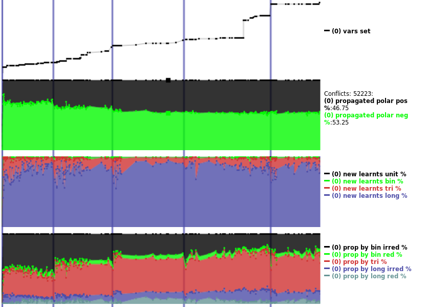
These graphs can show quite a bit of data, the above must be a few hundred data points. The data gathered is pumped to an SQL database, and then visualized. I felt like I am on to something. Finally, I was going to be able to explain things.

But I was able to explain very little. Some things were quite obvious, like how industrial and cryptographic instances’ variable polarity distributions were so different. Above, the black/green graph shows a cryptographic instance, and the distribution is 47% vs. 53%. On a typical industrial instance, the same graph looks like:

Here, the polarity distribution is 6% vs 94%. This is easy to see with the human eye. But I was gathering tons more data, many megabytes per instance. What was I going to do with all this data? How was I going to know what is good and bad behavior? And how would I make the solver work towards good?

SATZilla: Solver Selection Using Machine Learning

I wasn’t the only one trying to make sense of SAT-related data and improve solving based on it. SATZilla has done this before. There, the idea was to gather information — called features — about the input CNF problem, run multiple SAT solvers, save how much time it took for the solver to run, then create code that matches the CNF features to the preferred SAT solver. This creates a lines like:

num-vars  num-clauses  Best Solver
132       16730        Lingeling
375       46741        CryptoMiniSat
834       41690        CryptoMiniSat

Where the first N columns are the features and the last column is the label that we calculated to be correct. SATZilla uses many features, such as the number of horn clauses, the ratio of variables and clauses, etc. Once such a table has been built, with lines called labeled training examples, it uses a machine learning system, for example Decision Trees, to classify (i.e. guess) which SAT solver would be best for any CNF instance. So it generalizes, and can guess which SAT solver is best for a CNF it has never seen.

This system is interesting but has some drawbacks. First, for each data line one must run 5-10 SAT solvers on a CNF, potentially using up to 20-30’000 CPU seconds. Hence, each labeled training example is extremely expensive. If you know about the Big Data hype, you know that spending $2 on a single data point is not viable. Modern systems use millions of labeled training examples to learn a classifier. Secondly, this system was not designed to work in an industrial setting, where the CNF is not presented in a single file but piece-by-piece through a library interface.

Enter DRAT

DRAT is a system used to verify the resolution proof that modern SAT solvers generate. Basically, every unsatifiable problem that SAT solvers solve can be shown to be unsatisfiable through a set of operations called resolutions, that eventually lead to the equation 0=1, which is trivially false. A DRAT verifier can know exactly which clause was used by the SAT solver at exactly which time during the creation of the proof. Hence, DRAT knows a lot. It can actually tell, after the solving has finished, which parts of the SAT solving were absolutely useless, and which ones useful. A resolution proof with thousands of resolutions can be computed in seconds, which means cheap data.

When I first really understood DRAT, I realized, what if I could get all this data out of DRAT, and use it as a label for the millions of data points I already have? I have finally found a label, available at a huge scale, to train on.

The Beginnings of CrystalBall

What to train for was still a question that needed answering. Since DRAT is so intimately connected with learnt clauses, I decided to train for throwing away as many unneeded learnt clauses as possible. This would definitely make solving faster, by throwing away everything that is useless weight and making sure everything that is useful stays.

I must thank Marijn Heule who helped me with the first hack of DRAT-trim in early 2016 to get data out from from it. I hacked CryptoMiniSat to add Clause IDs to DRAT, so the verifier, DRAT-trim, could read and track these IDs. I now knew which clause was used in the proof and which wasn’t. This sounds really useful — you could now know which learnt clauses should have been thrown away the moment they were generated, since they were useless. Let’s see some data from modern CrystalBall (see at the bottom of the post how to download, compile and run):

sqlite> select count() from sum_cl_use where num_used>0;
51675

sqlite> select count() from sum_cl_use where num_used=0;
42832

The data says that about 50% of clauses were useful. Let’s see what is the average LBD value of the useful and useless clauses:

sqlite> select avg(glue) from sum_cl_use, clauseStats where sum_cl_use.clauseID = clauseStats.clauseID and num_used > 0;
6.71436865021771

sqlite> select avg(glue) from sum_cl_use, clauseStats where sum_cl_use.clauseID = clauseStats.clauseID and num_used = 0;
9.80162028389989

Nice. Let’s get the sizes, too, by replacing “glue” with “size”:

sqlite> select avg(size)...
12.2770198355104
sqlite> select avg(size)...
23.5734497571909

Cool. Size is a better discriminator? Let’s see another feature. Let’s get the average LBD of the redundant non-binary antecedents of the clause:

sqlite> select avg(antecedents_glue_long_reds_avg)...
4.88254061122689
sqlite> select avg(antecedents_glue_long_reds_avg)...
5.68082216847043

There are plenty more, well over a hundred, that is being measured, so I won’t bore you. I have a feeling you could write a few research papers just by running queries on this data.

I don’t know if you noticed, but something is odd here. SAT solvers only keep about 5-10% of all clauses. Just run a modern SAT solvers to completion and check how many clauses remain in the clause database. How is this compatible with 50% of clauses being useful? Well, we can use clauses for a while, then throw them away. But for that, we need much more than just whether a clause is useful or not. We need to know exactly when it was useful. Clauses can be used many-many times in a single proof.

We Need More Refined Labels

It turns out that having only whether a clause is being used is not good enough to compute useful labels. We need to know when, exactly, was the clause useful. So CryptoMiniSat and DRAT-trim was hacked to output into the DRAT proof exact conflict numbers when a clause was created. This, with some minor magic, would tell us exactly when each learnt clauses was used:

sqlite> select sum(num_used) from sum_cl_use, clauseStats where sum_cl_use.clauseID = clauseStats.clauseID and glue<=3;
332689

sqlite> select count() from clauseStats where glue<=3;
11221

For this problem, a clause that had LBD 3 or lower was used on average 332689/11221.0=29.65 times in the proof. Okay, how about clauses with LBD 4 or larger? It’s a trivial change in the above code, and gives us 5.95. Cool, the lower glue, the more it’s used in the proof.

Now that we know how to walk, let’s run. When was clauseID 59465 created and at what conflict points was it used in the proof?

sqlite> select conflicts from clauseStats where clauseID=59465;
101869

sqlite> select used_at from usedClauses where clauseID = 59465 order by used_at asc;
101870
123974
152375

This is an interesting clause. It was generated at conflict no. 101869, was used in the proof right after it was generated, at conflict no. 101870, and then it was used in the proof more than 20’000 conflicts later, twice.

The Data Pipeline

The idea is this: we are going examine every learnt clause at every 10’000 conflicts, and guess whether it’s going to be used in the future enough for it to be kept. If it’s going to be used enough in the future, we keep it. If not, we’ll throw it away. What do we need for this?

Well, we need a ton of labeled training examples. And for that, we need a truckload of data, one that generates so much that we have to throw away 96% and still end up with hundreds of MBs in under an hour. Also, we need this from a wide variety of problems, and we need to be able to debug the hell out of this data, because where there is tons of data, there are tons of NaNs, and negative clause sizes and the whatnot. So we need a data pipeline.

The first part of the pipeline we only run once, because it’s a bit expensive, about 3-10x slower than a normal CNF run, and looks like this:

  1. Run CryptoMiniSat without any clause cleaning, and write an SQLite database with all dynamic data gathered. The data written is about: the CNF (such as number of claues, etc.), the restarts (e.g. avg. LBD, restart length), the learnt clauses (e.g. LBD, size), and at every 10’000 conflicts the dynamic characteristics of the learnt clauses (e.g. activity, number of times used in a conflict the past 10’000 conflicts)
  2. Run DRAT, and dump all usage data to a file. Augment the SQLite data with the DRAT data
  3. Sample the data because otherwise it’s going to be too much. We need to sample smartly, though, because without biased sampling, the really weird cases will not be represented in the final data at all, and our machine learning system will not see some really interesting data. If we could store and process 1TB of data (you can generate that rather easily), we wouldn’t have this issue. But we can’t.

So now we have a ton of cool data that is very raw. This is going to be our baseline. We’ll keep this data in our stash and never modify it.

The second part of our data pipeline will use this stash of data to do all the cool things we want. This 2nd part is much-much cheaper to run (few seconds to a few minutes per CNF), so we will be able to run it as many times as we like, playing with all the cool parameters. This second part of the pipeline will:

  1. The data is stored normalized in SQLite for speed and space. For machine learning, we must denormalize it, to have everything related to decision on a single line.
  2. Create the labeled training data using Python Pandas for easy data manipulation and visualization
  3. Create a classifier using Python’s scikit-learn
  4. Spit out a C++ code we can compile into our solver

Getting Labeled Training Examples

In order to train a classifier, we need labeled training examples. These are lines like:

glue   size  used_last_10k_conflicts  activity rank   label
10     15     3                       top half        KEEP
7      10     1                       bottom half     THROW_AWAY
3      7      0                       bottom half     THROW_AWAY

Notice that this table has essentially two parts. The left part, i.e. everything apart from “keep”, called features, must be available to the solver during running. And the right part, “keep”, the label, which is computed using data from DRAT-trim. This latter the solver has no access to during running, this is our crystal ball, looking into the future. What we want is to predict the label given the features.

The left hand side, i.e. the features are not so difficult to do. Adding a new feature is now about 3-4 lines change in CryptoMiniSat and it’s essentially free in terms of speed. The data gathering only needs to run once (the 1st part of our data pipeline) and it is not running during solving. So, you can add as many features as you like. If they are useful, then you also need to add some lines to the solver so they will be available during running — of the 200+ only a few are really useful.

The right hand side, i.e. the labels are a completely different story, though. We know what is the future, kinda (yes, the future is a function of the past&present, but let’s not go there for the moment). So given the future, how do I label things? We need to use a heuristic. The good part is that we have a ton of information about the future, such as the distribution of all clause’s usage in the proof, and the number of times a particular clause is used in the future. But we still need to come up with something to decide KEEP/THROW_AWAY. A simple such heuristic is: if in the next 10’000 conflicts this clause will be used at least 6 times, keep it. Otherwise, into the bin it goes:

CASE WHEN
-- useful in the next round
   used_later10k.used_later10k > 5

THEN "keep" ELSE "throw_away"
END AS `x.class`

Nice! Remember that clauseID 59465 that I talked about above? Yeah, that would be labeled THROW_AWAY — it was only used 20’000 conflicts later. We have labeled our data, now we need to train a classifier, make it output C++ code and we are good to go. But before that, let’s play with Weka.

Data Analysis And Machine Learning with Weka

Weka is a cool tool for exploring data and building simple classifiers. You can get a free Weka course on Futurelearn, and I highly recommend it. The person who wrote it is the one who is giving the course and he is really cool. The denormalized, labeled data can be output to CSV (see at the bottom), which Weka can read:
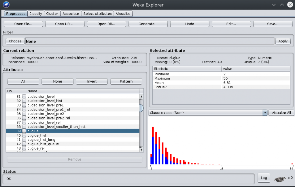
Here, you have Weka showing the denormalized set of features on the left, and showing the LBD distribution on the right. Blue color is for for lines labeled KEEP and red color is for lines labeled THROW_AWAY. As you can see, the distribution of blue vs red is not the same at all as the LBD value increases (hence LBD being a good discriminator, see glucose).

You can also visualize correlations:
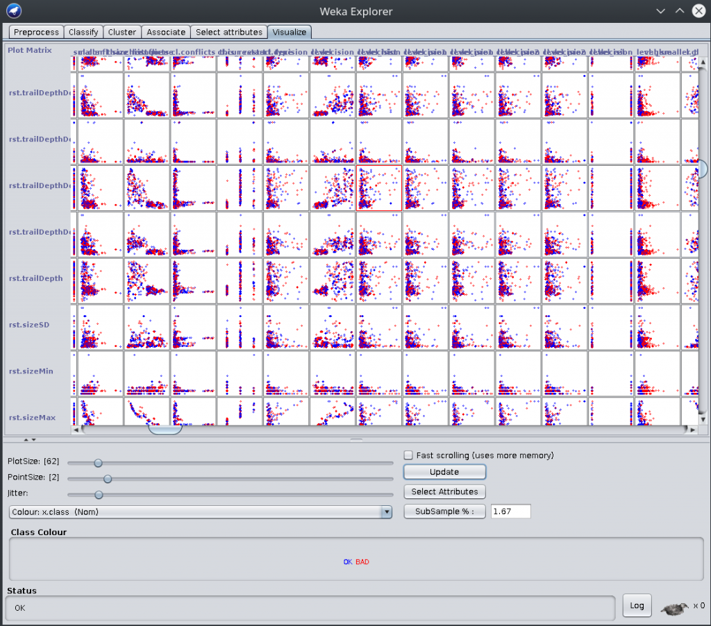
You can also build classifiers based on this labeled data. Just don’t forget to delete the “sum_cl_use.*” features, as they are not really features, they are data from the proof verification. If you don’t delete them, Weka will cheat and use them in the classifier, which is like using the solution key during the exam :) Let’s create a classifier using Weka:
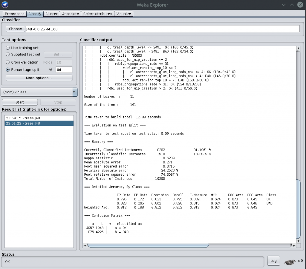
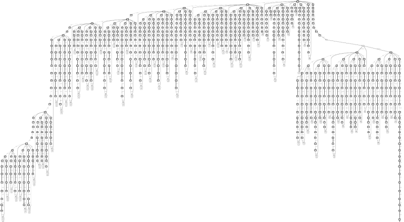
This shows a confusion matrix at the bottom. Nice. Total misclassification was 18% using the J48 decision tree algorithm with some minor tuning. Here is such an example decision tree (PDF here):

Weka is great in many ways, and I will forever be indebted to it. However, it’s just not gonna cut it for us. We need something a lot faster, and we need to be able to automate it and we need to be able to get C++ code out. Weka could do some of these, but I’m not a Java programmer, and Weka’s speed is nowhere near that of scikit-learn. However, if it’s your first time doing machine learning, Weka is an amazing tool.

Training a Classifier Using scikit-learn

Now that we have labeled training data, we need to create a classifier so that the solver, during running, can take the features it knows and guess the label KEEP or THROW_AWAY. There are many-many different classifiers that can be trained, and I have tried the most important ones, such as logistic regression, SVM, decision trees and random forests.

Let me pause here for a moment. If you haven’t done machine learning before, you might think — this is where the magic is. The classifier is where it’s at! And if you have done machine learning before, you know full well, it’s not here at all. It turns out that the quality and quantity of your data is way more important than the classifier you choose. It’s relatively easy to see why. If your data is messy, incorrect, or missing elements, no matter what classifier you use, no matter how amazing it is, it will give you bad results. Bad data, bad results. Every. Single. Time. Keep this in mind.

So, we have chosen our classifier, say, decision trees. Decision trees are easy to visualize, and you will need to debug the hell out of this, so it comes handy. After all, nobody wrote 1000 lines of python and it came out perfect the first time.

Now, there are still some things to deal with. First, we cannot possibly use all 200+ features in our prediction. We can generate the tables, but we need to be reasonable, and cut down the features to something much smaller, say, 20, during the running of the solver. To do that, we create a large random forest and then check which features were picked by the most trees. That gives us feature ranking (thanks to Raghav Kulkarni for this trick):

../predict.py "mydata-min.db-short-conf-0.dat" --name short
[...]
Feature ranking:
1 rdb0.used_for_uip_creation 0.1070
2 rdb0.last_touched_diff     0.0723
3 rdb0.act_ranking           0.0694
4 rdb0.activity_rel          0.0644
5 rdb0.sum_uip1_used         0.0641

So the top 5 features for this particular run are these. For different instances or different configurations, the top features may differ, and you probably want to sample X number of labeled training example from each problem, put it in a large data file and then run the feature ranking.

There are still some minor obstacles to overcome. Since about 95% of the clauses need to be thrown away, our labels will be very unbalanced. So we need to balance that. Also, how aggressive do we want to be with throwing clauses away? Should we err on the side of caution? Note that this is not about labeling anymore. The label has already been chosen. It’s about guessing the label. We are now tuning what’s called the confusion matrix:

X          label     label
           KEEP      THROW_AWAY

guessed    0.80      0.20
KEEP

guessed    0.05      0.95
THROW_AWAY

Here, we have 80% of things that we labeled as KEEP actually being guessed to be kept, while 20% of them are wrongly guessed as THROW_AWAY. So it’s kinda okay. We are better at guessing if something needs to be thrown away, though, there we only guess 5% of them wrongly. Maybe this a good balance, but if not, it can be changed as a weight parameter.

The system can also classify clauses into different types, using K-means clustering. Then it can train a different classifier for each clause type. The K-means clustering uses the already denormalized features, so it’s really trivial to do, though which features should be used for the clustering is a good question. I currently use the CNF features only (e.g. number of clauses, variables, ratio of vars/clauses, etc.), thereby clustering problems rather than clauses. One could could use any set of features though, it’s all automatic, including C++ code generation.

Actually, the C++ code generation. The system produces C++ code for decision trees, random forests and K-means clustering, ready for it to be compiled into the final executable. We have now created our clustering and classifier, and it’s all in C++ code. Let’s run it!

The Final Solver

This is the most fun part. And the cumulative effort of a lot of work. It’s really interesting to see all those thousands of lines of C++ and python churning out gigabytes of data, being boiled down to juts a few hundred lines of automatically generated if-then-else statements, running during solving. But there it is.

Let me talk about the good parts first. It’s very fast at evaluating whether to keep or throw away a clause. You don’t even notice it running. It doesn’t use much more memory than normal CryptoMiniSat (i.e. a few features were enough), and it correctly guesses the cluster where a clause belongs. It also guesses the labels correctly with very high probability. The final solver beats every solver from 2018 on the SAT competition 2014-17 instances.

Another great thing is that this system can be used to automatically train for specific problem types. This can be very significant in industry, where the instances are similar and training for a particular type of instance would make a lot of sense. Since this system tunes to the data it’s given, if it’s given data only about a particular type of instances, it will tune to them only, making the solver particularly good at them.

There is a bad part too, though: the built-in, rather sophisticated heuristic of keeping or throwing away clauses beats the system built. This makes me very sad, but some things make me hopeful. Firstly, the data is probably still messy. There are probably some bugs here and there, where some of the data gathered is not reliable. Secondly, the labeling is very-very rudimentary. If you have a look at that CASE statement above, it’s laughingly simple. Finally, the normal heuristic is quite smart, keeping some (simple) information about clauses, i.e. keeping some state over time, which the current machine learning system cannot do — the classifier has no memory.

Conclusions

This project, going back over 6 years, has been a tough one. All in all, it must have costed about 2 full years of work. A sane researcher would have abandoned it after about 2 weeks. In fact, we had a reviewer rejecting the paper, claiming that this work could be done in 2 weeks by her/his PhD student (I love such reviews). I sometimes wonder how much that PhD student charges for their time, because I might just pay it if they are that good.

Maybe we did the wrong thing, keeping going for so many years, but I think this could be a foundation of something much more interesting. It could be used not only to create machine learning models, but also to understand SAT solvers. With so much data at hand, we could finally understand some of the behavior of solvers, perhaps leading to some interesting ideas. And the data could be used for many other machine learning systems, too: guessing when to restart, guessing which variable to branch on, etc.

Build and Use Instructions

# Prerequisites on a modern Debian/Ubuntu installation
sudo apt-get install build-essential cmake git
sudo apt-get install zlib1g-dev libsqlite3-dev
sudo apt-get install libboost-program-options-dev 
sudo apt-get install python3-pip
sudo pip3 install sklearn pandas numpy lit matplotlib

# Getting the code
git clone https://github.com/msoos/cryptominisat
cd cryptominisat
git checkout crystalball
git submodule update --init
mkdir build && cd build
ln -s ../scripts/crystal/* .
ln -s ../scripts/build_scripts/* .

# Let's get an unsatisfiable CNF
wget https://www.msoos.org/largefiles/goldb-heqc-i10mul.cnf.gz
gunzip goldb-heqc-i10mul.cnf.gz

# Gather the data, denormalize, label, output CSV,
# create the classifier, generate C++,
# and build the final SAT solver
./ballofcrystal.sh --csv goldb-heqc-i10mul.cnf
[...compilations and the full data pipeline...]

# Let's use our newly built tool
# we are using configuration number short:3 long:3
./cryptominisat5 --predshort 3 --predlong 3 goldb-heqc-i10mul.cnf
[ ... ]
s UNSATISFIABLE

# Let's look at the data
cd goldb-heqc-i10mul.cnf-dir
sqlite3 mydata.db
sqlite> select count() from sum_cl_use;
94507
SAT Solvers as Smart Search Engines

Satisfiability problem solvers, or SAT solvers for short, try to find a solution to decidable, finite problems such as cryptography, planning, scheduling, and the like. They are very finely tuned engines that can be looked at in two main ways . One is to see them as proof generators, where the SAT solver is building a proof of unsatisfiability as it runs, i.e. it tries to prove that there is no solution to the problem. Another way is to see SAT solvers as smart search engines. In this blog post, I’ll take this latter view and try to explain why I think intermediary variables are important. So, for the sake of argument, let’s forget that SAT solvers sometimes restart the search (forgetting where they were before) and learn clauses (cutting down the search space and remembering where not go again). Let’s just pretend all they do is search.

Searching

The CryptoMiniSat SAT solver used to be able to generate graphs that show how a search through the search space went. Search spaces in these domains are exponential in size, say, 2^n in case there are n variables involved. I don’t have the search visualization code anymore but below is an example of such a search tree. The search starts at the very top not far from the middle, it descends towards the bottom left, then iteratively backtracks all the way to the top, and then descends towards the bottom right. Every pentagon at the bottom of a line is a place where the SAT solver backtracked. Observe that it never goes all the way back to the top — except once, when the top assignment needs to be flipped. Instead, it only goes back some way, partially unassigning variables. The bottom right corner is where the solution is found after many-many partial backtracks and associated partial unassignements:

What I want you to take away from this graph is the following: the solver iteratively tries to set a variable a value, calculates forward, and if it doesn’t work, it will partially backtrack, flip its value to its opposite, then descend again.

Brute force search vs. SAT solving

Trying one value and then trying the other sounds suspiciously like brute force search. Brute force search does exactly that, in a systematic and incredibly efficient way. We can build highly specialized executables and even hardware, to perform this task. If you look at e.g. Bitcoin mining, you will see a lot of specialized hardware, ASICs, doing brute-force search. And if you look at rainbow tables, you’ll see a lot of bit slicing.

So why waste our time doing all this fancy value propagation and backtracking when we could use a much more effective, systematic search system? The answer is, if you generated your problem description wrongly, then basically, for no good reason, and you are probably better off doing brute-force search. But if you did well, then a SAT solver can perform a significantly better search than brute-force. The trick lies in intermediary variables, and partial value assignments.

Partial value assignments

So let’s say that your brute force engine is about to check one input variable setting. It sets the input variables, runs the whole algorithm, and computes the output. The output is wrong though. Here is where things go weird. The brute force engine now completely erases its state, takes another input and runs the whole algorithm again. 

So, brute force does the whole calculation again, starting from a clean state, every time. What we have to recognize is that this is actually a design choice. Another design choice is to calculate what variables were affected by one of the input bits, unset these variables, flip the input bit value, and continue running the calculation. This has the following requirements:

  1. A way to quickly determine which intermediate values depend on which other ones so we can unset variables and know which intermediate, already calculated, dependent variables also need to be unset.
  2. A way to quickly unset variables
  3. A good set of intermediary values so we can keep as much state of the calculation as possible

If you think about it, the above is what SAT solvers do, well mostly. In fact, they do (1) only partially: they allow variables only to be unset in reverse chronological order. Calculating and maintaining a complete dependency graph seems too expensive. So we unset more variables than we need to. But we can unset them quickly and correctly and we compensate for the lack of correct dependency check in (1) by caching polarities. This caches the independent-but-nevertheless-unset variables’ values and then hopes to reassign them later to the correct value. Not perfect, but not too shabby either.

Modeling and intermediary variables

To satisfy requirement (3) one must have a good set of intermediary variables in the input problem (described in DIMACS format), so the SAT solver can both backtrack and evaluate partially. Unfortunately, this is not really in the hands of the SAT solver. It is in the hands of the person describing the problem. Modeling is the art of transforming a problem that is usually expressed in natural language (such as “A person cannot be scheduled to be on a night shift twice in a row”) into a problem that can be given to a SAT solver.

Modeling has lots of interesting constraints, one of which I often hear and I am confused by: that it should minimize the number of variables. Given the above, that SAT solvers can be seen at as partial evaluation engines that thrive on the fact that they can partially evaluate and partially backtrack, why would anyone try to minimize the number of variables? If the solver has no intermediary variables to backtrack to, the solver will simply backtrack all the way to the beginning every time, thus becoming a really bad brute-force engine that incidentally tracks a dependency graph and is definitely non-optimized for the task at hand.

Some final thoughts

In the above I tried to take a premise, i.e. that SAT solvers are just search engines, and ran with it. I don’t think the results are that surprising. Of course, nothing is black-and-white. Having hundreds of millions of variables in your input is not exactly optimal. But minimizing the number of variables given to a SAT solver at the expense of expressive intermediate variables is a huge no-no.

Clause glues are a mystery to me

Note: the work below has been done in collaboration with Vegard Nossum, but the wording and some of the (mis-)conculsions are mine. If you are interested, check out his master thesis, it’s quite incredible

Anyone who has ever tried to really understand clause glues in SAT solvers have probably wondered what they really mean. Their definition is simple: the number of variables in the final conflict clause that come from different decision levels. An explanation of these terms can be found here. On the surface, this sounds very simple and clean: the number of different decision levels should somehow be connected to the number of variables that need to be set before the learnt clause activates itself, i.e. it causes a propagation or a conflict. Unfortunately, this is just the surface, because if you try to draw 2-3 implication graphs, you will see that in fact the gap between the number of variables needed to be set (let’s call this ‘activation number’) and the glue can be virtually anything, making the glue a potentially bad indicator of the activation number.

The original reasoning

The original reasoning behind glues is the following: variables in the same decision level, called ‘blocks of variables’ have a chance to be linked together through direct dependencies, and these dependencies should be expressed somehow in order to reduce the number of decisions needed to reach a conflict (and thus ultimately reduce the search space). To me, this reasoning is less clear than the one above. In fact, there are about as many intuitions about glues as the number of people I have met.

Glucosetrack

With Vegard Nossum we have developed (in exactly one day) something quite fun. On the face of it, it’s just glucose 1.0, plain and simple. However, it has an option, “-track”, which does the following: whenever a learnt clause is about to cause a conflict, it jumps over this learnt clause, saves the state of the solver, and works on until the next conflict in order to measure the amount of work the SAT solver would have had to do if that particular learnt clause had not been there. Then, when the next clause wishes to cause a conflict, it records the amount of propagation and decisions between the original conflict and this new conflict, resets the state to the place saved, and continues on its journey as if nothing had happened. The fun part here is that the state is completely reset, meaning that the solver behaves exactly as glucose, but at the same time it records how much search that particular cause has saved. This is very advantageous because it doesn’t give some magical number like glue, but actually measures the usefulness of the given clause. Here is a typical output:

c This is glucose 1.0  with usefulness tracking by
c Vegard Nossum and Mate Soos. Based on glucose, which
c is in run based on MiniSat, Many thanks to all teams
c
c ============================[ Problem Statistics ]=============================
c |                                                                             |
c |  Number of variables:  138309                                               |
c |  Number of clauses:    942285                                               |
c |  Parsing time:         0.28         s                                       |
============================[ Search Statistics ]==============================
| Conflicts |          ORIGINAL         |          LEARNT          | Progress |
|           |    Vars  Clauses Literals |    Limit  Clauses Lit/Cl |          |
===============================================================================
|         0 |  138309   942285  2636352 |   314095        0   -nan |  0.000 % |
|       620 |  138074   942285  2636352 |   314095      615     82 |  1.559 % |
|       919 |  135307   925938  2596895 |   314095      906     75 |  3.908 % |
|      2714 |  130594   894562  2518954 |   314095     2664     67 |  6.799 % |
|      2814 |  130593   894562  2518954 |   314095     2763     69 |  6.808 % |
|      2930 |  130592   894562  2518954 |   314095     2879     70 |  6.808 % |
|      4042 |  127772   874934  2471045 |   314095     3974     69 |  9.292 % |
|      4142 |  127772   874934  2471045 |   314095     4074     70 |  9.292 % |
...
c Cleaning clauses (clean number 0). Current Clause usefulness stats:
INSERT INTO data(cleanno, idx, size, glue, conflicts, props, bogoprops, decisions) VALUES(0 , 961074 , 107 , 5 , 42 , 185509 , 1301341 , 0);
INSERT INTO data(cleanno, idx, size, glue, conflicts, props, bogoprops, decisions) VALUES(0 , 944729 , 14 , 1 , 7 , 36865 , 268229 , 0);
INSERT INTO data(cleanno, idx, size, glue, conflicts, props, bogoprops, decisions) VALUES(0 , 948275 , 7 , 1 , 15 , 27909 , 220837 , 0);
INSERT INTO data(cleanno, idx, size, glue, conflicts, props, bogoprops, decisions) VALUES(0 , 953762 , 102 , 2 , 2 , 29365 , 197410 , 0);
...
c End of this round of database cleaning
...
|     38778 |  110896   758105  2182915 |   314095    28270     93 | 20.167 % |
|     39488 |  110894   758105  2182915 |   314095    28978     93 | 20.185 % |
c Cleaning clauses (clean number 1). Current Clause usefulness stats:
INSERT INTO data(cleanno, idx, size, glue, conflicts, props, bogoprops, decisions) VALUES(1 , 979236 , 71 , 1 , 8 , 45531 , 280156 , 0);
INSERT INTO data(cleanno, idx, size, glue, conflicts, props, bogoprops, decisions) VALUES(1 , 954908 , 2 , 2 , 7 , 0 , 232760 , 0);
...

The output is in SQL format for easy SQL import. The “size” is the clause size, “glue” is the glue number, “conflicts” is the number of times the clause caused a conflict, “props” is the number of propagations gained by having that clause (i.e. by doing the conflict early), “bogoprops” is an approximation of the amount of time gained based on the number of watchlists and the type of clauses visited during propagation, and “decisions” is the number of decisions gained. The list is sorted according to “bogoprops”, though once the output is imported to MySQL, many sortings are possible. You might notice that the ‘glue’ is 1 for some clauses (e.g. on the second output line) — these are clauses that have caused a propagation at decision level 0, so they will eventually be removed through clause-cleaning, since they are satisfied. Notice that high up, there are some relatively large clauses (of size 102 for example) with glue 2, that gain quite a lot in terms of time of search. The gained conflicts/propagations/etc. are all cleared after every clause-cleaning, though since clauses are uniquely indexed (‘idx’), they can be accumulated in all sorts of ways.

The program is 2-5x slower than normal glucose, but considering that it has to save an extreme amount of state due to the watchlists being so difficult to handle and clauses changing all the time, I think it does the job quite well — as a research tool it’s certainly quite usable. In case you wish to download it, it’s up in GIT here, and you can download a source tarball here. To build, issue “cmake .” and “make”. Note that the tool only measures the amount of search saved by having the clause around when it tries to conflict. It does not measure the usefulness of the propagations that a learnt clause makes. Also, it doesn’t measure the other side of the coin: the (potentially better) conflict generated by using this clause instead of the other one. In other words, it gives a one-sided view (no measure of help through propagation) of a one-sided view (doesn’t measure the quality of difference between the conflict clauses generated). Oh well, it was a one-day hack.

Experiments

I have made very few experiments with glucosetrack, but you might be interested in the following result. I have taken UTI-20-10p0, ran it until completion, imported the output into MySQL, and executed the following two queries. The first one:

SELECT glue, AVG(props), FROM data
WHERE glue >= 2 AND size >= 2
GROUP BY glue
ORDER BY glue

calculates the average number of saved propagations between each round of cleaning for clauses of glue >= 2 (i.e. clauses that didn’t eventually cause a propagation at decision level 0), and of size >= 2, because unitary clauses are of no interest. The second is very similar:

SELECT size, AVG(props), FROM data
WHERE glue >= 2 AND size >= 2
GROUP BY size
ORDER BY size

which calculates the same as above, but for size.

Some explanation is in order here regarding why I didn’t count SUM(), and instead opted for AVG(). In fact I personally did make graphs for SUM(), but Vegard corrected me: there is in fact no point in doing that. If I came up with a new glue calculation function that gave an output of ‘1’ for every clause, then the SUM for that function would look perfect: every clause would be in the same bracket, saving a lot of propagations, but that would not help me make a choice of which clauses to throw out. But the point of glues is exactly that: to help me decide which clauses to throw out. So what we really want is a usefulness metric that tells me that if I keep clauses in that bracket, how much do I gain per clause. The AVG() gives me that.

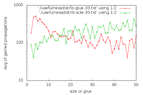
Here goes the AVG() graph for the last clause cleaning (clause cleaning iteration 33):

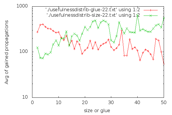
Notice that the y axis is in logscale. In case you are interested in a larger graph, here it is. The graph for clause cleaning iteration 22 is:

(Iteration 11 has high fluctuations due to less data, but for the interested, here it is). I think it’s visible that glues are good distinguishers. The graph for glues drops down early and stays low. For sizes, the graph is harder to read. Strangely, short clauses are not that good, and longer clauses are better on average. If I had to make a choice about which clauses to keep based on the size graph, it would be a hard choice to make: I would be having trouble selecting a group that is clearly better than the rest. There are no odd-one-out groups. On the other hand, it’s easier to characterise which clauses are good to have in terms of glues: take the low glue ones, preferably below 10, though we can skip the very low ones if we are really picky. An interesting side-effect of the inverse inclination of the size and glue graphs and the fact that “glue<=size” is that maybe we could choose better clauses to keep if we go for larger clauses that have a low glue.

Conclusions

Unfortunately, there are no real conclusions to this post. I guess running glucosetrack for far more than just one example, and somehow also making it measure the difference between the final conflict clauses’ effectiveness would help to write some partially useful conclusion. Vegard and me have tried to put some time and effort into this, but to not much avail I am afraid.

PS: Notice that glucosetrack allows you to generate many of the graphs here using the right SQL query.

Collecting solver data

Lately, I have been putting a lot of effort into collecting data about solver behaviour and dumping it on-the-fly to a MySQL database. Some of this data is then presented by a PHP&javascript interface, such as this.The goal is to better understand how solving works, and thus to possibly come up with better strategies for solving. The requirements of the data gathered are: speed to calculate, size to store and usefulness.

Gathered data

There are some obvious statistics that one would like to collect, such as number of conflicts, propagations and conflicts per second, etc — these are all gathered by almost every SAT solver out there. However, it would be interesting to have more. Here is what CryptoMiniSat now gathers and dumps using highly efficient prepared bulk insert statements, using at most 5% of time.

For each variable, dumped once in a while:

  • no. times propagated false, and true (separately)
  • no. times decided false and true (sep.)
  • no. times flipped polarity
  • avg & variance of decision level
  • avg & variance of propagation level

For each clause larger than 3-long, dumped once in a while:

  • activity
  • conflict at which it was introduced (if learnt)
  • number of propagations made
  • number of conflicts made
  • number of times any of its literal was looked at during BCP
  • number of times it was looked at (dereferenced) during BCP
  • number of times used to resolve with during learnt clause generation
  • number of resolutions needed to during its generation (if learnt clause)

For earch restart:

  • no. of reducible&irreducible (i.e. learnt&non-learnt) binary clauses
  • no. of red&irred tertiary clauses (separately)
  • no. of red&irred long clauses (sep)
  • avg, variance,  min and max of learnt clause glues
  • avg, var, min, max of learnt clause sizes
  • avg, var, min, max of number of resolutions for 1st UIP
  • avg,var,min,max of branch depths
  • avg,var,min,max of backjump length –in the number of literals unassigned
  • avg,var,min,max of backjump lenght — in the number of levels backjumped
  • avg, var, min, max times a conflict followed a conflict without decisions being made
  • avg,var,min,max of agility
  • no. of propagations by red&irred binary clauses
  • no. of props by red&irred tertiary clauses
  • no. of props by red&irred long clauses
  • no. of conflicts by red&irred binary clauses (separately)
  • no. of conflicts by red&irred tertiary clauses (sep)
  • no. of conflicts by red&irred  long clauses (sep)
  • no. of learnt unit, binary, tertiary, and long clauses (sep)
  • avg,var, min,max of watchlist size traversed during BCP
  • time spent
  • no. of decisions
  • no. of propagations
  • no. of variables flipped
  • no. of variables set positive&negative (sep)
  • no. of variables currently unset
  • no. of variables currently replaced
  • no. of variables currently eliminated
  • no. of variables currently set

For each learnt clause database cleaning:

  • for reducible clauses removed: all the data in the “clauses larger than 3-long” data above, summed up
  • for reducible clauses not removed: all the data in the “clauses larger than 3-long” data above, summed up
  • no. of clauses removed
  • no. of clauses not removed
  • for all irred clauses (these are not touched): all the data in the “clauses larger than 3-long” data above, summed up

For every N conflicts:

  • clause size distribution
  • clause glue distribution
  • clause size and glue scatter data

This is all, and is not all mine. Suggestions were made by many, some as much as a year ago: George Katsirelos, Luca Melette, Vegard Nossum, Valentin-Mayer Eichberger, Ben Schlabs,  Said Jabbour and Niklas Sörensson. Naturally, none of these people necessarily approve of how I gather data or what I do with the data gathered, but they helped, so listing them is only fair.

What’s not yet or cannot be gathered

Two suggestions are still on the TODO list:

  • counting the number of conflicts done while a learnt clause was “locked”, i.e. has propagated in the current search tree. This stat of a learnt clause could tell us if the clause seemed essential to the search or not. If a clause propagated once, at the bottom of the search tree, and then the variable propagated was quickly unset, it’s not the same as if the same clause propagated at the top of the search tree, and then the variable it set was essentially never unset.
  • for each variable, counting the number of conflicts done while the variable was set. This is interesting, because if a variable was propagated only once, at top-level, it will seem like it was never set (set only once), yet it may have had a huge influence on the search tree and consequently on the learnt clauses.

Both of these require a change in the algorithm used to backjump and although I am a bit worried about the performance, I will add these soon.

Unfortunately, the data about variables can’t really be dumped so often, because it’s huge for large problems with millions of variables. So I guess I will only dump that for the most active N variables, for some sane definition of “active”. Similarly, the data about individual clauses is not dumped, only in a summed-up way during database cleaning.

Suggestions?

In case you have any ideas what else could be interesting to dump, please put it as a comment. The idea is to dump data that is cheap to compute and cheap to dump yet would be interesting for some reason or another. I am prepared to add stuff to datastructures, as you have probably guessed from the above. Yes, it makes the clause database less space-efficient, and so increases cache-miss. But on large problems, it’s going to be a cache-miss most of the time anyway, and a cache-fetch brings in 128B of data, which should be plenty for both the stats and the clause. Similarly with variables. So, don’t refrain from suggesting some stuff that takes space. Also, weird stuff is interesting. The most weird stat on the list above is definitely the “conflict after a conflict without decisions” (suggested by Said Jabbour) which I would have guessed to be zero, or near-zero, yet is pretty high, in the 30+% range.

Suggestions are welcome!

Visualizing SAT solving

Visualizing the solving of mizh-md5-47-3.cnf


Visualizing what happens during SAT solving has been a long-term goal of mine, and finally, I have managed to pull together something that I feel confident about. The system is fully explained in the liked image on the right, including how to read the graphs and why I made them. Here, I would like to talk about the challenges I had to overcome to create the system.

Gathering information

Gathering information during solving is challenging for two reasons. First, it’s hard to know what to gather. Second, gathering the information should not affect overall speed of the solver (or only minimally), so the code to gather the information has to be well-written. To top it all, if much information is gathered, these have to be structured in a sane way, so it’s easy to access later.

It took me about 1-1.5 months to write the code to gather all information I wanted. It took a lot of time to correctly structure and to decide about how to store/summarize the information gathered. There is much more gathered than shown on the webpage, but more about that below.

Selecting what to display, and how

This may sound trivial. Some would simply say: just display all information! But what we really want is not just plain information: what good is it to print 100’000 numbers on a screen? The data has to be displayed in a meaningful and visually understandable way.

Getting to the current layout took a lot of time and many-many discussions with all all my friends and colleagues. I am eternally grateful for their input — it’s hard to know how good a layout is until someone sees it for the first time, and completely misunderstands it. Then you know you have to change it: until then, it was trivial to you what the graph meant, after all, you made it!

What to display is a bit more complex. There is a lot of data gathered, but what is interesting? Naturally, I couldn’t display everything, so I had to select. But selection may become a form of misrepresentation: if some important data isn’t displayed, the system is effectively lying. So, I tried to add as much as possible that still made sense. This lead to a very large table of graphs, but I think it’s still understandable. Further, the graphs can be moved around (just drag their labels), so doing comparative analysis is not hampered much by the large set of graphs.

The final layout is much influenced by Edward Tufte‘s books. Most graphic libraries for javascript, including what I used, Dygraphs, contain a lot of chartjunk by default. For example, the professional library HighCharts is full chartjunk (just look at their webpage), and is apparently used by many Fortune 500 companies. I was appalled at this — many-many graph libraries, none that offers a clean look? Luckily, I could do away with all that colorful beautifying mess — the data is interesting, and demands no embellishments.

Creating the webpage

Creating the webpage to display what I wanted was quite difficult. I am no expert at PHP or HTML, and this was the first time I had touched javascript. Although the final page doesn’t show it much, I struggled quite a bit with all these different tools. If I had to do this again, I would choose to use a page generation framework. This time, I wrote everything by hand.

I am most proud of two things on the webpage. First is the histogram at the bottom of the graphs. I know it may not seem like it, but that is all done with a javascript I wrote that pulls data from an array that could be dynamically changed. I think it does what it’s supposed to do, and does it well. The second is that I had to tweak the graph library used (Dygraphs, the best library out there, hands down), because it was too slow at printing these ~30 graphs. The graphs can be zoomed (just click and drag on X axis), and when zooming in&out the speed was really terrible. It now works relatively fast though I had to tweak the system to trade speed for a bit of visual beauty.

Final thoughts

Making the visualization webpage was a long marathon. I feel like it’s OK now, even though there were quite a number of ideas that weren’t implemented in the end. I hope you will enjoy playing with it as much as I have enjoyed making it.