Tag Archives: SAT

The Inprocessing API of CryptoMiniSat

Many modern SAT solvers do a lot of what’s called inprocessing. These steps simplify the CNF into something that is easier to solve. In the compiler world, these are called rewritngs since the effectively rewrite (parts of) the formula to something else that retain certain properties, such as satisfiability. One of the most successful such rewrite rules for CNF is Bounded Variable Elimination (BVE, classic paper here), but there are many others. These rewrites are usually done by modern SAT solvers in a particular order that was found to be working well for their particular use-case, but they are not normally accessible from the outside.

Sometimes one wants to use these rewrite rules for something other than just solving the instance via the SAT solver. One such use-case is to use these rewrite rules to simplify the CNF in order to count the solution to it. In this scenario, the user wants to rewrite the CNF in a very particular way, and then extract the simplified CNF. Other use-cases are easy to imagine, such as e.g. MaxSAT, core counting, etc. Over the years, CryptoMiniSat has evolved such a rewrite capability. It is possible to tell CryptoMiniSat to simplify the formula exactly how the user wants the solver to be satisfied and then extract the simplified formula.

Example Use-Case

Let’s say we have a CNF that we want to simplify:

p cnf 4 2
1 2 3 4 0
1 2 3 0

In this CNF, 1 2 3 4 0 is not needed, because it is subsumed by the clause 1 2 3 0. You can run subsumption using CryptoMiniSat this way:

#include "cryptominsat5/cryptominisat.h"
#include <vector>
#include <cmath>
#include <iostream>

using namespace CMSat;
using namespace std;
#define lit(a) Lit(std::abs(a)-1, a<0)

int main() {
  Solver s;
  vector<Lit> cl;
  s.add_new_vars(4);

  cl = vector<Lit>{lit(1), lit(2), lit(3), lit(4)};
  s.add_clause(cl);
  cl = vector<Lit>{lit(1), lit(2), lit(3)};
  s.add_clause(cl);
  
  s.simplify(NULL, "occ-backw-sub");
  s.start_getting_clauses();
  while(s.get_next_clause(cl) {
    for(const auto l: cl) cout << l << " ";
    cout << endl;
  }
  s.end_getting_clauses()
  
  return 0;
}

This code runs the inprocessing system occ-backw-sub, which stands for backwards subsumption using occurrence lists. The input CNF can be anything, and the output CNF is the simplified CNF. This sounds like quite a lot of code for simple subsumption, but this does a lot of things under the hood for things to be fast, and it is a lot more capable than just doing subsumption.

Notice that the first argument we passed to simplify() is NULL. This means we don’t care about any variables being preserved — any variable can (and will) be eliminated if occ-bve is called. In case some variables are important to you not to be eliminated, you can create a vector of them and pass the pointer here. If you have called the renumber API, then you can get the set of variables you had via clean_sampl_and_get_empties(). The numbering will not be preserved, but their set will be the same, though not necessarily the same size. This is because some variables may have been set, or some variables may be equivalent to other variables in the same set. You can get the variables that have been set via get_zero_assigned_lits().

Supported Inprocessing Steps

Currently, the following set of inprocessing steps are supported:

API nameInprocessing performed
occ-backw-subBackwards subsumption using occurence lists
occ-backw-sub-strBackwards subsumption and strengthening using occurence lists
occ-bceBlocked clause elimination (paper)
occ-ternary-resTernary resolution (paper)
occ-lit-remLiteral removal via strengthening
occ-cl-rem-with-orgatesOR-gate based clause removal (unpublished work, re-discovered by others)
occ-rem-with-orgatesOR-gate based literal removal
occ-bveBounded variable elimination (paper)
occ-bve-emptyBounded variable elimination of empty resolvents only
intree-probeProbe using in-tree probing, also do hyper-binary resolution and transitive reduction (paper). Also does hyper-binary resoution & transitive reduction
full-probeProbe each literal individually (slow compared to intree-probe)
backboneBackbone simplification (cadiback paper)
sub-implSubsume with binary clauses with binary clauses (fast)
sub-str-cls-with-binSubsume and strengthen long clauses with binary clauses (fast)
sub-cls-with-binSubsume long clauses with binary clauses (fast)
distill-binsDistill binary clauses
distill-clsDistill long clauses (distillation paper)
distill-cls-onlyremDistill long clauses, but only remove clauses, don’t shorten them. Useful if you want to make sure BVE can run at full blast after this step.
clean-clsClean clauses of set literals, and delete satisfied clauses
must-renumberRenumber variables to start from 0, in case some have been set to TRUE/FALSE or removed due to equivalent literal replacement.
must-scc-vreplPerform strongly connected component analysis and perform equivalent literal replacement.
oracle-vivifyVivify clauses using the Oracle tool by Korhonen and Jarvisalo (paper). Slow but very effective.
oracle-vivif-sparsifyVivify & sparsify clauses using the Oracle tool by Korhonen and Jarvisalo. Slow but very effective.

Convenience Features Under the Hood

The steps above do more than what they say on the label. For example, the ones that start with occ build an occurrence list and use it for the next simplification stop if it also starts with occ. They also all make sure that memory limits and time limits are adhered to. The timeout multiplier can be changed via set_timeout_all_calls(double multiplier). The time limits are entirely reproducible, there is no actual seconds, it’s all about an abstract “tick” that is ticking. This means that all bugs in your code are always reproducible. This helps immensely with debugging — no more frustrating Heisenbugs. You can check the cryptominisat.h file for all the different individual timeouts and memouts you can set.

Under the hood you also get a lot of tricks implemented by default. You don’t have to worry about e.g. strengthening running out of control, it will terminate in reasonable amount of ticks, even if that means it will not run to completion. And the next time you run it, it will start at a different point. This makes a big difference in case you actually want your tool to be usable, rather than just “publish and forget”. In many cases, simplification only makes things somewhat faster, and you want to stop performing the simplification after some time, but you also want your users to be able to report bugs and anomalies. If the system didn’t have timeouts, you’d run the risk of the simplifier running way too long, even though the actual solving would have taken very little time. And if the timeout was measured in seconds, you’d run the risk of a bug being reported but being irreproducible, because the exact moment the timeout hit for the bug to occur would be irreproducible.

Making the Best of it All

This system is just an API — it doesn’t do much on its own. You need to play with it, and creatively compose simplifications. If you take a look at cryptominisat.h, it already has a cool trick, where it moves the simplified CNF from an existing solver to a new, clean solver through the API, called copy_simp_solver_to_solver(). It is also used extensively in Arjun, our CNF simplifier for counting. There, you can find the function that controls CryptoMiniSat from the outside to simplify the CNF in the exact way needed. It may be worthwhile reading through that function if you want to control CryptoMiniSat via this API.

The simplify() API can give you the redundant clauses, too (useful if you e.g. did ternary or hyper-binary resolution), and can give you the non-renumbered CNF as well — check out the full API in cryptominisat.h, or the Arjun code. Basically, there is a red and a simplified parameter you can pass to this function.

Perhaps I’ll expose some of this API via the Python interface, if there is some interest for it. I think it’s quite powerful and could help people who use CNFs in other scenarios, such as MaxSAT solving, core counting, core minimization, etc.

Closing Thoughts

I think there is currently a lack of tooling to perform the already well-known and well-documented pre- and inprocessing steps that many SAT solvers implement internally, but don’t expose externally. This API is supposed to fill that gap. Although it’s a bit rough on the edges sometimes, hopefully it’s something that will inspire others to either use this API to build cool stuff, or to improve the API so others can build even cooler stuff. While it may sound trivial to re-implement e.g. BVE, once you start going into the weeds of it (e.g. dealing with the special case of detecting ITE, OR & AND gates’ and their lower resolvent counts, or doing it incrementally with some leeway to allow clause number increase), it gets pretty complicated. This API is meant to alleviate this stress, so researchers and enthusiasts can build their own simplifier given a set of working and tested “LEGO bricks”.

Checking Uniform-Like Samplers

Uniform sampling is pretty simple: there are a set of solutions to a set of equations, and I want you to give me N solutions uniformly at random. Say, I have a set of equations that only has the solutions x=1…6, and I ask you to give me solutions uniformly at random. In this case, if the system is not cheating, it should give me solutions exactly like a random dice would give: 1..6, each with the same probability of 1/6. Now, if you give me nothing but 1’s I’d be slightly confused, and eventually would think you may be trying to cheat.

Uniformity is useful not only in gambling, but also e.g. if you want to make sure to cover a good chunk of the potential states in a system. Say, your equations describe how a program can run. Now, uniform solutions to these equations will be examples of the state space of your program. If you want to check that your system is in most cases doing the right thing, you can ask for uniform solutions at random and check the states for inconsistencies or unexpected behaviors.

Uniform Sampling of CNFs

One type of equations that is quite popular is to have all variables boolean (i.e. True/False), and equations being nothing but an “AND of ORs”, i.e. something like: “(a OR b) AND (b OR c OR d) AND (-f OR -g)”. These types of equations, also known as CNF, can express quite complicate things, e.g. (parts of) computer programs, logical circuits (e.g. parts of CPUs), and more. What’s nice about CNF is that there are many different tools to convert your problem language into CNF.

Given CNF as the intermediate language, all you need to do is run a uniform sampler on the CNF, and interpret the samples given your transformation. For example, you could translate your Ethereum cryptocurrency contract into QF_BV logic and blast that to CNF using e.g. the STP solver. Then you can get uniform random examples of the execution of your cryptocurrency contract using e.g. UniGen.

There are many different samplers for CNFs, and they mostly fall into two categories: ones that give guarantees and are hence truly uniform, and ones that don’t give guarantees and therefore fall into what we’ll call uniform-like samplers. These latter samplers tend to be significantly faster than truly uniform samplers, however, they can, and sometimes do, give non-uniform samples. I personally help maintain one truly uniform sampler, UniGen (PDF), and one uniform-like sampler, CMSGen (PDF). Other popular truly uniform samplers include KUS (PDF) and SPUR (PDF).

Catching Uniform-Like Samplers: Barbarik

If I give you a sampler and ask you to tell me if it’s truly uniform or simply uniform-like, what should you do? How should we distinguish one from the other, without looking into the internals of the system? It turns out that this is not a simple question to answer. It is very reasonable to assume that there are e.g. 2^200 solutions, so e.g. trying to prove that a sampler is uniform by saying that it should only output the same sample twice rarely is not really meaningful. In this latter case, you’d need to get approx 2^100 samples from a truly uniform sampler before it will likely give two colliding samples. While a uniform-like sampler may collide at e.g. only 2^60 (i.e. a trillion times earlier), that’s still a lot of computation, and only a single data point.

Doing this efficiently is the question that was on the minds of the authors of Barbarik. Basically, their idea was the following: take a CNF, remove all solutions but two, and blow up these two solutions into equally many solutions each. Say, you find two solutions to a CNF, one BLUE and one RED. Barbarik will take BLUE, make 100 blue balls out of it, and take RED, and make 100 red balls out of it. Then, it will give the CNF with the 200 solutions, half blue, half red, to the sampler under test. Then it asks the sampler to give it a bunch of balls. We of course expect approx 50%-50% red-blue distribution of balls from a truly uniform sampler.

Barbarik fails a solver if it is gives a distribution too far away from the 50%-50% we’d expect. Barbarik runs this check many times, with different example blue/red solutions that are “blown up” to multiple solutions. Given different base CNFs, and many tries, it is possible to differentiate the good from the bad… most of the time:

If you take a look at the table above, QuickSampler and STS, both uniform-like samplers, are rejected by Barbarik given 50 different CNFs. In contrast, UniGen survives all 50 tests with flying colors. Notice, however, that CMGen also survived all tests.

The Birth of CMSGen

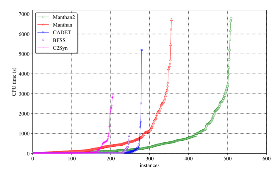
When Barbarik was being created, I was fortunate enough to be present, and so I decided to tweak my SAT solver, CryptoMiniSat purely using command-line parameters, until Barbarik could not distinguish it from a truly uniform sampler. This, in my view, showcased how extremely important a test system was: I actually had a bug in CryptoMiniSat’s randomization that Barbarik clearly showed and I had to fix to get higher quality samples. We called the resulting uniform-like sampler CMSGen, and it was used in the function synthesis tool Manthan (PDF), that blew all other function synthesis system out of the water, thanks to its innovative design and access to high quality, fast samples from CMSGen:

Notice that within 200 seconds Manthan outperformed all other function synthesis systems, even if we give the other system 7000 seconds to work with. If you are interested in the details of this crazy improvement over previous state-of-the-art, check out the slides here or the video here (these are all work of my coworkers, I am not an author).

While CMSGen was clearly fast and powerful, it bothered me endlessly that Barbarik couldn’t demonstrate that it wasn’t a truly uniform sampler. This eventually lead to the development of ScalBarbarik.

The Birth of ScalBarbarik

Since CMSGen passed all the tests of Barbarik, we had to come up with a new trick to distinguish it from truly uniform samplers. ScalBarbarik‘s (PDF) underlying system is still the same as Barbarik: we take a CNF, take 2 samples from it, and blow both of these samples up to a certain number. However, how we blow them up is where the trick lies. Before, they were both blown up the same way into solutions that are equally easy/hard to find. However, this time around, we’ll make one of the solution types much harder to find than the other. For this, we’ll use Vegard Nossum’s SHA-1 CNF generator (PDF) to force the system to reverse a partial, reduced-round SHA-1 hash, with some fixed inputs & outputs. This allows us to both change the complexity of the problem and the number of solutions to it rather easily.

While one set of solutions will be hard to find, the other ones will be trivial to find — if one special variable is set to TRUE, the finding a set of solutions is trivial But when it’s set to FALSE, the system has to reverse a reduce-round SHA-1. The logic behind this is that the uniform-like systems will likely be finding the easy solutions with much higher probability than the hard solutions, so they will sample much more unevenly. Indeed that’s the case:

Note that as the hardness parameter is increased, CMSGen is rejected more and more often, and eventually it’s rejected for all CNFs. Also interesting to note is that QuickSampler and STS get both rejected, as before, but this time around, STS gets rejected for all 50 CNFs, rather than for only 36 out of 50. In other words, ScalBarbarik is overall a stronger/better distinguisher.

Conclusions

With the birth of Barbarik, a set of uniform-like testers were shown to be less than ideal, and a new, more robust near-uniform sampler was born, CMSGen. But as a the gauntlet has been throw down by CMSGen, a new tool emerged, ScalBarbarik, to help find the non-truly uniform samplers. With this cycle in mind, I hope that new, more elaborate, and higher-quality uniform-like samplers will emerge that will be able to beat ScalBarbarik at its own game, improving the quality of the sampling while maintaining the speed advantage that uniform-like samplers enjoy over truly uniform samplers. With better uniform-like sampling tools, hopefully we’ll be able to make headway in automated test case generation (imagine having it as part of all development IDEs), higher performance function synthesis, and hopefully even more diverse areas of interest for the general public.

CryptoMiniSat 5.6.3 Released

The latest CryptoMiniSat, version 5.6.3 has been released. This release marks the 12’000th commit to this solver that has weathered more than I originally intended it to weather. It’s been an interesting ride, and I have a lot to thank Kuldeep and NSCC‘s ASPIRE-1 cluster for this release. I have burned over 200k CPU hours to make this release, so it’s a pretty well-performing release (out-performing anything out there, by a wide margin), though I’m working very hard to make sure that neither I nor anyone else will have to burn anything close to that to make a well-performing SAT solver.

The solver has some interesting new algorithms inside, the most interesting of which is Gauss-Jordan elimination using a Simplex-like method, generously contributed by Jie-Hong Roland Jiang and Cheng-Shen Han from the National Taiwan University. This addition should finally settle the issues regarding Gaussian vs Gauss-Jordan elimination in SAT solvers. Note that to use this novel system, you must configure with “cmake -DUSE_GAUSS=ON ..” and then re-compile.

What’s also interesting is what’s not inside, though. I have been reading (maybe too much) Nassim Taleb and he is very much into via negativa. So I tried removing algorithms that have been in the solver for a while and mostly nobody would question if they are useful. In the end I removed the following algorithms from running by default, each removal leading to better solving time:

  • Regular probing. Intree probing is significantly better, so regular probing is not needed. Thanks Matti/Marijn/Armin!
  • Stamping. This was a big surprise, especially because I also had to remove caching, which is my own, crappy (“different”) version of stamping. I knew that it wasn’t always so good to have, but damn. It was a hard call, but if it’s just slowing it down, what can I do. It’s weird.
  • Burst searching. This is when I search for a short period with high randomness all over the search space. I thought it would allow me to explore the search space in places where VSIDS/Maple doesn’t. Why this is slowing the solver down so much may say more about search heuristics/variable bumping/clause bumping than anything.
  • Note that I never had blocked clause elimination. It doesn’t work well for incremental solving. In fact, it doesn’t work at all, though apparently the authors have some new work that allows it to work, super-interesting!

I’m nowadays committed to understanding this damned thing rather than adding another impossible-to-explain magic constant  to make the solving 10% faster. I think there is interesting stuff out there that could be done to make SAT solvers 10x, not 10%, faster.

CryptoMiniSat 3.0 released

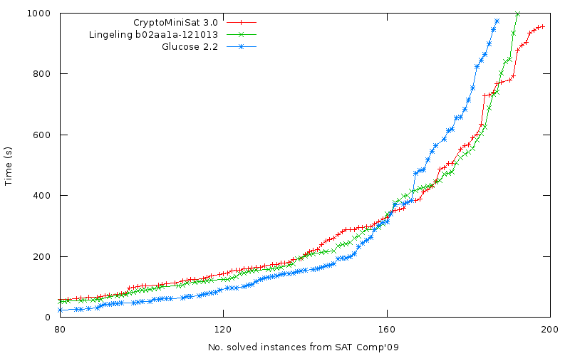
CryptoMiniSat 3.0 has been released. I could talk about how it’s got a dynamic, web-based statistics interface, how it has more than 80 options, how it uses no glues for clause-cleaning and all the other goodies, but unfortunately these don’t much matter if the speed is not up to par. So, here is the result for the 2009 SAT Competition problems on a 1000s timeout with two competing solvers, lingeling and glucose:

cryptoms_speed

This of course does not mean that CryptoMiniSat is faster than the other solvers in general. In fact it is slower on a number of instances. What it means is that in general it’s OK and that’s good enough for the moment. It would be awesome to run the above experiment (or a similar one) with a longer timeout. Unfortunately, I don’t have a cluster to do that. However, if you have access to one, and would be willing to help with running the 3 solvers on a larger timeout, please do, I will post the updated graph here.

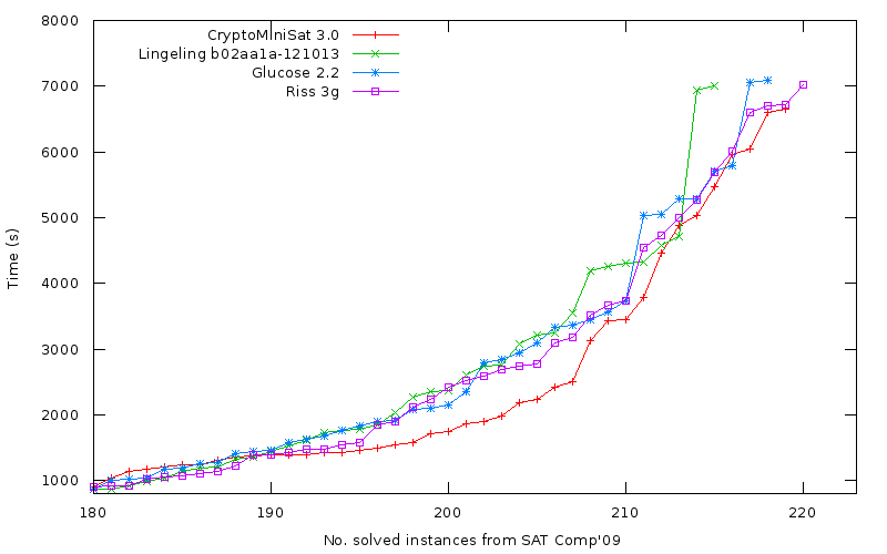
Update Norbert Manthey kindly ran all the above solvers on the TU Dresden cluster, thanks! He also kindly included one more solver, Riss 3g. The cluster was an AMD Bulldozer architecture with 2cores/solver with an extreme, 7200s timeout. The resulting graph is here:

cryptoms_speed

Riss 3g is winning this race, with CryptoMiniSat being second, third is glucose, and very intriguingly lingeling the 4th. Note that CryptoMiniSat leads the pack most of the time. Also note, this is the first time CryptoMiniSat 3.0 has been run for such a long time, while all the other competing solvers’ authors (lingeling, glucose, riss) have clusters available for research purposes.

Licensing

For those wondering if they could use this as a base for SAT Competition 2013, the good news is that the licence is LGPL so you can do whatever you want with it, provided you publish the changes you made to the code. However, I would prefer that you compete with a name such as “cms-MYNAME” unless you change at least 10% of the code, i.e. ~2000 lines. For the competitions after 2013, though, it’s all up for grabs. As for companies, it’s LGPL, so you can link it with your code, it’s safe, you only have to publish what you change in the library, you don’t have to publish your own code that uses the library.

Features

CryptoMiniSat has been almost completely rewritten from scratch. It features among other things:

  • 4 different ways to propagate
  • Implicit binary&tertiary clauses
  • Cached implied literals
  • Stamping
  • Blocking of long clauses
  • Extended XOR detection and top-level manipulation
  • Gate detection and manipulation
  • Subsumption, variable elimination, strengthening
  • 4 different ways to clear clauses
  • 4 different ways to restart
  • Large amounts of statistics data, both into console and optionally to MySQL
  • Web-based dynamic display of gathered statistics
  • 3 different ways to calculate optimal variable elimination order
  • On-the-fly variable elimination order update
  • Super-fast binary&tertiary subsumption&strengthening thanks to implicit bin&tri
  • On-the-fly hyper-binary resolution with precise time-control
  • On-the-fly transitive reduction with precise time-control
  • Randomised literal dominator braching
  • Internal variable renumbering
  • Vivification
  • On-the-fly clause strengthening
  • Cache&stamp-based learnt clause minimisation
  • Dynamic strongly connected component check and equivalent literal replacement

Code layout

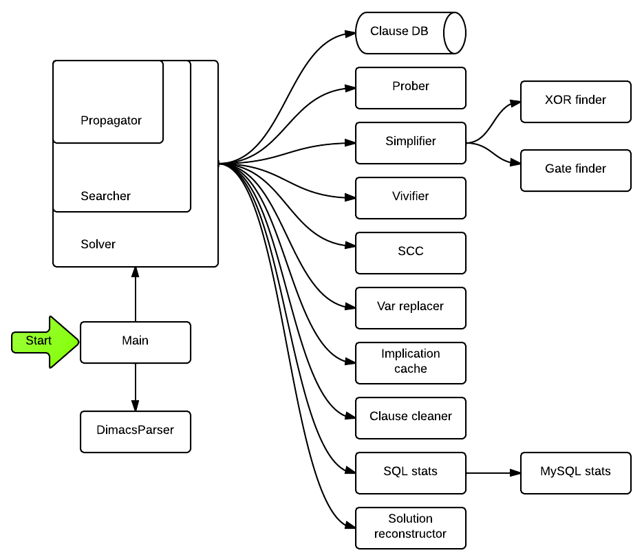
As for those wondering how large the code base is, it’s about 20KLOC of code, organised as:

cryptoms_overview

Visualizing SAT solving

Visualizing the solving of mizh-md5-47-3.cnf


Visualizing what happens during SAT solving has been a long-term goal of mine, and finally, I have managed to pull together something that I feel confident about. The system is fully explained in the liked image on the right, including how to read the graphs and why I made them. Here, I would like to talk about the challenges I had to overcome to create the system.

Gathering information

Gathering information during solving is challenging for two reasons. First, it’s hard to know what to gather. Second, gathering the information should not affect overall speed of the solver (or only minimally), so the code to gather the information has to be well-written. To top it all, if much information is gathered, these have to be structured in a sane way, so it’s easy to access later.

It took me about 1-1.5 months to write the code to gather all information I wanted. It took a lot of time to correctly structure and to decide about how to store/summarize the information gathered. There is much more gathered than shown on the webpage, but more about that below.

Selecting what to display, and how

This may sound trivial. Some would simply say: just display all information! But what we really want is not just plain information: what good is it to print 100’000 numbers on a screen? The data has to be displayed in a meaningful and visually understandable way.

Getting to the current layout took a lot of time and many-many discussions with all all my friends and colleagues. I am eternally grateful for their input — it’s hard to know how good a layout is until someone sees it for the first time, and completely misunderstands it. Then you know you have to change it: until then, it was trivial to you what the graph meant, after all, you made it!

What to display is a bit more complex. There is a lot of data gathered, but what is interesting? Naturally, I couldn’t display everything, so I had to select. But selection may become a form of misrepresentation: if some important data isn’t displayed, the system is effectively lying. So, I tried to add as much as possible that still made sense. This lead to a very large table of graphs, but I think it’s still understandable. Further, the graphs can be moved around (just drag their labels), so doing comparative analysis is not hampered much by the large set of graphs.

The final layout is much influenced by Edward Tufte‘s books. Most graphic libraries for javascript, including what I used, Dygraphs, contain a lot of chartjunk by default. For example, the professional library HighCharts is full chartjunk (just look at their webpage), and is apparently used by many Fortune 500 companies. I was appalled at this — many-many graph libraries, none that offers a clean look? Luckily, I could do away with all that colorful beautifying mess — the data is interesting, and demands no embellishments.

Creating the webpage

Creating the webpage to display what I wanted was quite difficult. I am no expert at PHP or HTML, and this was the first time I had touched javascript. Although the final page doesn’t show it much, I struggled quite a bit with all these different tools. If I had to do this again, I would choose to use a page generation framework. This time, I wrote everything by hand.

I am most proud of two things on the webpage. First is the histogram at the bottom of the graphs. I know it may not seem like it, but that is all done with a javascript I wrote that pulls data from an array that could be dynamically changed. I think it does what it’s supposed to do, and does it well. The second is that I had to tweak the graph library used (Dygraphs, the best library out there, hands down), because it was too slow at printing these ~30 graphs. The graphs can be zoomed (just click and drag on X axis), and when zooming in&out the speed was really terrible. It now works relatively fast though I had to tweak the system to trade speed for a bit of visual beauty.

Final thoughts

Making the visualization webpage was a long marathon. I feel like it’s OK now, even though there were quite a number of ideas that weren’t implemented in the end. I hope you will enjoy playing with it as much as I have enjoyed making it.