Tag Archives: resolution

Why it’s hard to eliminate variables

Let’s examine why it’s hard to eliminate variables. I remember the code I looked at in SatElite that did it: it was crazy clean code and looked like it was pretty easy to perform. In this post I’ll examine how that simple code became more than a 1’000 lines of code today.

What needs to be done, at first sight

At first sight, variable elimination is easy. We just:

  1. Build occurrence lists
  2. Pick a variable to eliminate
  3. Resolve every clause having the positive literal of the variable with negative ones.
  4. Add newly resolved clauses into the system
  5. Remove original clauses.
  6. Goto 2.

These are all pretty simple steps at first sight, and one can imagine that implementing them is maybe 50-100 lines of code, no more. So, let’s examine them one-by-one to see how they get complicated.

Building occurrence lists

The idea is that we simply take every single clause, and for every literal they have, we insert a pointer to the clause into an array for that literal’s occurrences. This sounds easy, but what happens if we are given 1M clauses, each with 1000 literals on average? If you think this is crazy, it isn’t, and does in fact happen.

One option is we estimate the amount of memory we would use and abort early because we don’t want to run out of memory. So, first we check the potential size, then we link them in. Unfortunately, this means we can’t do variable elimination at all. Another possibility is that we link in clauses only partially. For example, we don’t link in clauses that are redundant but too long. Redundant clauses are ignored during resolution when eliminating, so this is OK, but then we will have to clean these clauses up later, when finishing up. However, if a redundant clause that hasn’t been linked in backward-subsumes an irredudant clause (and thus becomes irredundant itself), we have to link it in asap. Optimisation leads to complexity.

We don’t just want to link these clauses in to some random datastructure. I believe it was Armin Biere who put this idea into my head, or maybe someone else, but re-using watchlists for occurrence lists means we use our memory resources better: there won’t be so much fragmentation. Furthermore, an advanced SAT solver uses implicit binary & tertiary clauses, so those are linked in already into the watchlists. That saves memory.

Picking a variable to eliminate

The order in which you eliminate clauses is a defining part of the speed we get with the final solver. It is crucially important that this is done well. So, what can we do? We can either use some heuristic or precisely calculate the gain for each variable, and eliminate the best guess/calculated one first. These are both greedy algorithms but I think given the complexity of the task, they are the best at hand.

Using precise calculation is easy, we just resolve all the relevant clauses but don’t add the resolvents. It’s very expensive though. A better approach is to use a heuristic. Logically, clauses that have few literals in them are likely not to resolve such that they become tautologies. It’s unlikely that two binary clauses’ resolvent becomes a tautology. It’s however likely that large clauses become tautological once resolved. I take this into account when calculating elimination cost for variable. Since redundant clauses are linked in the occurrence lists so that I can subsume them, I have to skip them.

It’s not enough to calculate the heuristic once, of course. We have to re-calculate after every elimination — the playing field has changed. Thus, for every clause you removed, you have to keep in mind which variables were affected, and re-calculate the cost for each after every variable elimination.

Resolving clauses

The base is easy. We add literals to a new array of literls and mark the literals that have been added in a quick-lookup array. If the opposite of a literal is added, the markings tell us and we can skip the rest — the resolvent is tautological. Things get hairy if the clause is not tautological.

What if the new clause is subsumed by already-existing clauses? Should we check for this? This is called forward-subsumption, and it’s really expensive. Backward subsumption (which asks the question ‘Does this clause subsume others?’ instead of ‘Is this clause subsumed by others?’) would be cheaper, but that’s not the case here. We can thus try to subsume the clause only by e.g. binary&tertiary clauses and hope for the best.

What if the new clause can be subsumed by stamps? That’s easy to check for, but if the new clause was used to create the stamp, that would be a self-dependency loop and not adding the resolvent would lead to an incorrect result. We can use the stamps as long as the resolving clauses were not needed for the stamp: i.e. they are not binary clauses and on-the-fly hyper-binary resolution was used during every step of stamp generation. A similar logic goes for using the implication cache.

We could also virtually extend the clause with literals using watchlists/stamps/impl. cache and then try to subsume that virtual clause. I forgot what 3-letter acronym Biere et al. gave to this method (it’s one of the 12 on slide 25 here), but, except for the acronym, this idea is pretty simple. You take a binary clause, e.g. xV~y, and if x is in the newly created clause, but y and ~y is not, you add y to the clause. The clause is now bigger, so has a larger chance to be subsumed. You now perform forward subsumption as above, but with the extended clause. Also, take care not to subsume clauses with themselves, which, as you might imagine, can get hairy.

If all of this sounds a bit intricate, this is not even the difficult part. The difficult part is keeping track of time. Where of course by time I don’t actually mean seconds — I mean computation steps that you have to define one way or another and increment counters and set limits. Remember: all this has to be deterministic.

Doing all of the above with a small but complicated instance is super-fast, under 0.001s. With a weird instance where one single literal may occur in more than a million clauses, it can be very-very expensive even for one single try — over 100s. That’s about 5 orders of magnitude of difference. So, you have to be careful. The resolution we cannot skip, but we can abort it (and indicate it up in the call tree). Some of the others we can abort, but then the whole resolution has to be re-started. Some of the above is not critical at all, so you have to use a different time-limit for some, and mark them as too expensive, so at least the basic things get done. This gets complicated, because e.g. forward-subsumption you might want to re-use at other parts of the solver so you have to use a time-limit that isn’t global.

Adding the newly resolved clauses

Adding clauses is simple: we create and link them in. However, we can do more. Since backward-subsumption is fast, we can do that with the newly created clauses. Note that this means the newly created clause could subsume some of the original clauses it was created from — which means the resolvents should be pre-generated and kept in memory.

Another thing: since we know the new clause needs to be added, we might as well shorten it before in any way we can. At this point, we can make use of all the watchlists, stamps and implication cache we have to shorten the new clause: there are no problems with self-dependencies. It will pay off. However, note that shortening the clause before adding it means that we will have to reverse-shorten it later, when this clause might be part of a group of clauses that is touched by a new variable elimination round. So, we are working against ourselves in a way — especially because reverse shortening is pretty expensive and hairy as explained above.

Although this is obvious, but we still have to take care of time-outs. For example, if resolution took so much time that we are already out of time, we must exit asap and not worry about the resolvents. Don’t link, don’t remove, just exit. Time is of essence.

Removing the original clauses

Easy, just unlink them from the occurrence lists. I mean, easy if you don’t care about time, of course. Because unlinking is an O(N^2) operation if you have N clauses and all of them contain the same literal X — the N-long occurrence list of literal X has to be read and updated N times. So, we don’t do this.

First of all, a special case: the two occurrence lists of the variable we are removing can simply be .clear()-ed. It’s no longer needed. Secondly, we shouldn’t unlink clauses one-by-one. Instead, we should mark the clause as removed, and then not care about the clause later. Once variable elimination is finished, we do a sweep of all the occurrence lists and clauses and remove the clauses that have been marked. This means that e.g. forward and backward subsumption gets more hairy (we shouldn’t subsume with a clause that’s been marked as removed but is still in the occurrence list) but that O(N^2) becomes O(N) which for problems where N is large makes quite a bit of difference. Like, the difference of 100s vs. 10s for a the same exact thing.

The untold horrors

On top of what’s above, you might like to generate some statistics about what worked and what didn’t. You might like to dump these statistics to a database. You might like to not create resolutions that are not needed as the irreduntant clauses form an AND/ITE gate. Or multiple gates. You might like to eliminate only a subset of variables at each call so that you don’t make your system too sparse and thus reduce arc consistency. You might want to vary this limit based on the problem at hand. You might want to do many other things that are not detailed above.

Conclusions

Once I read through the above, I realized I kind of missed the essence: time-outs. It’s mentioned here and there, but it’s much more critical than it seems and makes things a hell of a lot harder. How do you cleanly exit from the middle of reverse-shortening while resolving because you ran out of time? I could just bury my head in sand of course and say: I don’t care. Or, I could make some messy algorithm that checks return values of each call and return a special value in case of time-outs. This needs to be done for every level of the call, which can be pretty deep, unless you like writing 1’500 line functions. I wanted to say writing&reading, but, really, nobody reads 1’500 line functions. They are throw-away,write-only code.
A note on learnt clauses

Learnt clauses are clauses derived while searching for a solution with a SAT solver in a CNF. They are at the heart of every modern so-called “CDCL” or “Conflict-Driven Clause-Learning” SAT solver. SAT solver writers make a very important difference between learnt and original clauses. In this blog post I’ll talk a little bit about this distinction, why it is important to make it, and why we might want to relax that distinction in the future.

A bit of terminology

First, let me call “learnt” clauses “reducible” and original clauses “irreducible”. This terminology was invented by Armin Biere I believe, and it is conceptually very important.

If a clause is irreducible it means that if I remove that clause from the clause database and solve the remaining system of constraints, I might end up with a solution that is not a solution to the original problem. However, these clauses might not be the “original” clauses — they might have been shortened, changed, or otherwise manipulated such as through equivalent literal replacement, strengthening, etc.

Reducible clauses on the other hand are clauses that I can freely remove from the clause database without the risk of finding a solution that doesn’t satisfy the original set of constraints. These clauses could be called “learnt” but strictly speaking they might not have been learnt through the 1st UIP learning process. They could have been added through hyper-binary resolution, they could have been 1UIP clauses that have been shortened/changed, or clauses obtained through other means such as Gaussian Elimination or other high-level methods.

The distinction

Reducible clauses are typically handled “without care” in a SAT solver. For example, during bounded variable elimination (BVE) resolutions are not carried out with reducible clauses. Only irreducible clauses are resolved with each other and are added back to the clause database. This means that during variable elimination information is lost. For this reason, when bounded variable addition (BVA) is carried out, one would not count the simplification obtained through the removal of reducible clauses, as BVE could then completely undo BVA. Naturally, the heuristics in both of these systems only count irreducible clauses.

Reducible clauses are also regularly removed or ‘cleaned’ from the clause database. The heuristics to perform this has been a hot topic in the past years and continue to be a very interesting research problem. In particular, the solver Glucose has won multiple competitions by mostly tuning this heuristic. Reducible clauses need to be cleaned from the clause database so that they won’t slow the solver down too much. Although they represent information, if too many of them are present, propagation speed grinds to a near-halt. A balance must be achieved, and the balance lately has shifted much towards the “clean as much as possible” side — we only need to observe the percentage of clauses cleaned between MiniSat and recent Glucose to confirm this.

An observation about glues

Glues (used first by Glucose) are an interesting heuristic in that they are static in a certain way: they never degrade. Once a clause achieves glue status 2 (the lowest, and best), it can never loose this status. This is not true of dynamic heuristics such as clause activities (MiniSat) or other usability metrics (CryptoMiniSat 3). They are highly dynamic and will delete a clause eventually if it fails to perform well after a while. This makes a big difference: with glues, some reducible clauses will never be deleted from the clause database, as they have achieved a high enough status that most new clauses will have a lower status (a higher glue) and will be deleted instead in the next cleaning run.

Since Glucose doesn’t perform variable elimination (or basically any other optimization that could forcibly remove reducible clauses), some reducible clauses are essentially “locked” into the clause database, and are never removed. These reducible clauses act as if they were irreducible.

It’s also interesting to note that glues are not static: they are in fact updated. The way they are updated, however, is very particular: they can obtain a lower glue number (a higher chance of not being knocked out) through some chance encounters while propagating. So, if they are propagated often enough, they have a higher chance of obtaining a lower glue number — essentially having a higher chance to be locked into the database.

Some speculation about glues

What if these reducible clauses that are locked into the clause database are an important ingredient in giving glues the edge? In other words, what if it’s not only the actual glue number that is so wildly good at guessing the usefulness of a reducible clause, instead the fact that their calculation method doesn’t allow some reducible clauses ever to be removed also significantly helps?

To me, this sounds like a possibility. While searching and performing conflict analysis SAT solvers are essentially building a chain of lemmas, a proof. In a sense, constantly removing reducible clauses is like building a house and then knocking a good number of bricks out every once in a while. If those bricks are at the foundation of the system, what’s above might collapse. If there are however reducible clauses that are never “knocked out”, they can act as a strong foundation. Of course, it’s a good idea to be able to predict what is a good foundation, and I believe glues are good at that (though I think there could be other, maybe better measures invented). However, the fact that some of them are never removed may also play a significant role in their success.

Locking clauses

Bounded variable addition is potentially a very strong system that could help in shortening proofs. However, due to the original heuristics of BVE it cannot be applied if the clauses it removes are only reducible. So, it can only shorten the description of the original problem (and maybe incidentally some of the reducible clauses) but not only the reducible clauses themselves. This is clearly not optimal for shortening the proof. I don’t know how lingeling performs BVA and BVE, but I wouldn’t be surprised if it has some heuristic where it treats some reducible clauses as irreducible (thereby locking them) so that it could leverage the compression function of BVA over the field of reducible clauses.

Unfortunately, lingeling code is hard to read, and it’s proprietary code so I’d rather not read it unless some licensing problems turn up. No other SAT solver performs BVA as an in-processing method (riss performs it only as pre-processing, though it is capable to perform BVA as in-processing), so I’m left on my own to guess this and code it accordingly.

UPDATE: According to Norbert Manthey lingeling doesn’t perform BVA at all. This is more than a little surprising.

End notes

I believe it was first Vegard Nossum who put into my head the idea of locking some reducible clauses into the database. It only occurred to me later that glues automatically achieve that, and furthermore, they seem to automatically lock oft-propagated reducible clauses.

There are some problems with the above logic, though. I believe lingeling increments the glue counter of some (all?) reducible clauses on a regular basis, and lingeling is a good solver. That would defeat the above logic, though the precise way glues are incremented (and the way they are cleaned) in lingeling is not entirely clear to me. So some of the above could still hold. Furthermore, lingeling could be so well-performing for other reasons — there are more to SAT solvers than just search and resolution. Lately, up to 50% or more of the time spent in modern SAT solvers could be used to perform actions other than search.

Failed literal probing and UIP

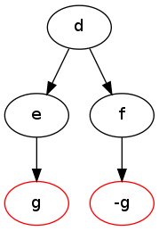
I have just realised that CryptoMiniSat, having won a number of medals, does one of the most basic things, failed literal probing, all wrong. Let me tell you why it’s all wrong. In essence, failed literal probing is trivial. We enqueue a fact, such as a, and then propagate it. If this fails, i.e. if two opposing facts such as g and -g are derived, we know that a cannot be true, so we set -a. Easy. Or maybe not so easy.

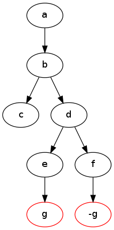
The devil is in the details, so let’s see how we derived both g and -g from a. Let’s assume that we have the following set of binary clauses:
-a V b
-b V c
-b V d
-d V e
-d V f
-e V g
-f V -g

which, from the point of view of a is best described as the graph:

Propagating "a", deriving both "g" and "-g"

The problem is, that if we only derive -a from this graph, we end up with only that one literal set, because -a doesn’t propagate anything on the clauses. This is quite sad, because, in fact, we could derive something stronger. From the graph it is evident that setting d would have failed: the graph would simply have its upper part cut away completely, but the lower part, including the derivation of both g and -g would still stand:

Deriving both "g" and "-g" from "d"

What is special about node d? Well, it’s where the 1st UIP, the first unique implication point, lies. And it is quite simple to see that -d is in fact the strongest thing we can derive from this graph. It’s much stronger than simply -a, because setting -d propagates on the clauses, giving -b,-a, setting three variables instead of one, including -a. An interesting observation is the following: deriving -b is the 2nd UIP, and deriving -a is the last UIP. In other words, at least in this most simple case, 1st UIP is in fact the strongest, and 2nd, 3rd.. last UIP are less strong in strict order.

Let me remark on one more thing about failed literal probing. Once failed literal probing has been done on literal x and it visited the node set N, there is no need to try to do failed literal probing on any nodes in N, since they cannot possibly fail. Although the failing of a literal can have consequences on the failing of other literals, if we ignore this side-effect, we could speed up failed literal probing by marking literals already visited, and only carrying out failed literal probing on ones that haven’t been marked. This is really trivial, but I haven’t been using it :S

I am quite sure that some advanced SAT solvers (such as lingeling) do all of the above things right. It’s probably only CryptoMiniSat that fails miserably :)

Note: there is a subtle bug with marking literals visited as “OK”. If two different subgraphs could fail, but we abort on the first one, then we might mark a literal OK when in fact it isn’t. It is therefore easiest not to mark any literals if the probe failed (which is very rare).

Fun facts about SAT solving (part 1)

Last time I gave a talk, I got some quite deserved fire about the way I approach SAT solving: in a more practical than scientific way. So, to give some food for thought for those who wish to approach SAT from a more scientific viewpoint, and to demonstrate to what lengths I have gone to give (at least to myself) a scientific viewpoint, let me talk a little bit about a fun fact that I have found. The fun fact, as is quite usual for SAT, seems entirely trivial, even banal, but has somehow (so far) eluded proper explanation for me. Maybe you will be the one to give the right explanation :)

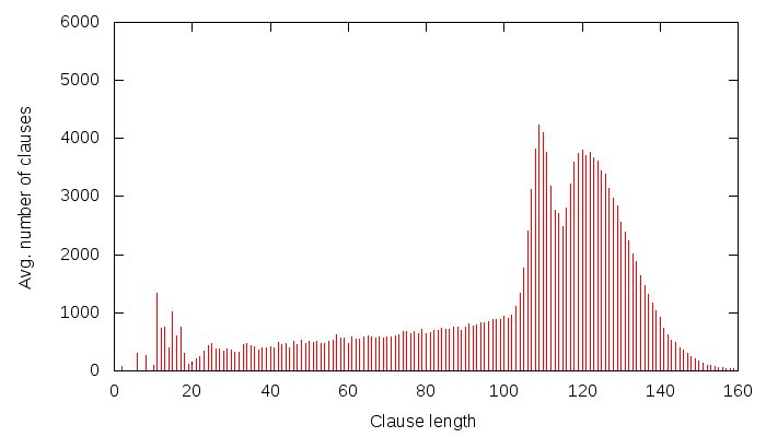
So, I generate a Grain cipher instance using, e.g. the Grain-of-Salt tool that I developed. If you don’t want to generate these yourself, there are a couple (multi-hundred thousand) pre-generated such problems you can download from here. I launch MiniSat 2.1 “core”(i.e. the most simple version) on these problems with a little twist: I write to a file the length of each generated learnt clause. Now, there are two kinds of CNF files I use: one that has 60 randomly picked randomly set state variables, and another one that is plain, and doesn’t have any variables set. Obviously, the CNF that has variables set should be easier to solve, and if Grain is a proper cipher, it should be about 2^60 easer to solve. Now, I print the average learnt clause length that I observe for the CNF that has 0 variables set, and I get this graph:

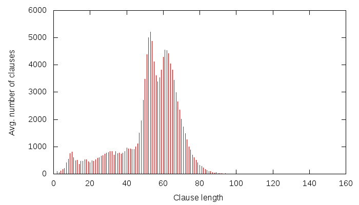
I am sure one could sing long and elaborate songs about this graph, but instead, I will just say: it has a strange curvy thing at around clause length 120. Now, I will generate a similar graph, but this time, I will use a CNF that has 60 state (i.e. important) variables set. Note that this should indeed be 2^60 times easier to solve (since Grain is a nice cipher, and my CNF generation abilities aren’t that poor). So the same graph for this CNF looks like this:

All right. This one, as I am sure you have noticed, has a curvy thing at around 60. Using elementary math, 120-60 = 60. Right, so one could reason: well, there were X unknowns, I have set 60 of them, now there are only X-60 left, so the average clause length should be 60 less! That I think doesn’t explain much, if anything, however. First off, the number of unknowns were in fact 160 — that’s the unknown state of Grain that we were trying to solve. Second, the learnt clauses don’t only contain state variables… in fact, a lot of variables they contain are not state variables at all! Furthermore, why should the 1st UIP scheme be so exact about clause sizes? After all, it’s just a graph-analysis algorithm working at the local conflict — it has no clue about the problem it is working with, much less about the number of state bits set in our instance of Grain.

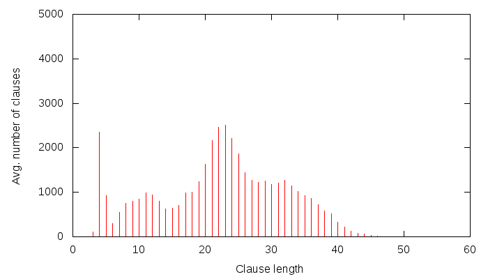
One could say that this is just a dumb example, and it has no real meaning. Maybe I just stumbled upon it, after all, 120/2 = 60, etc. However, this doesn’t seem to be the case. I can, in fact, reproduce this for a lot of X’s for any of the following ciphers: Grain, Trivium, Bivium, HiTag2 and Crypto-1. Let me show one from HiTag2. Again, we are solving for the state, and we don’t set any state bits (i.e. this is the full HiTag2 problem):

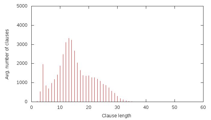
Okay, there is a bumpy thing at around 23. Now, let’s set 10 randomly picked state variables to random values, and run the example again:

There seems to be a bumpy thing at around 13. 23-10 = 13. That’s about right.

By the way, I have stumbled upon the above fun fact about 2 years ago (well before CryptoMiniSat was born), when working on my diploma thesis — these graphs are actually taken verbatim from my thesis. I have worked a lot on SAT in the past 2 years, but this has been haunting me ever since. Maybe someone could explain it to me?

PS: Does anyone know if someone has done an in-depth analysis of learnt clause length distributions, maybe even three-dimensional, showing the time on the Z axis? It would be awesome to do that, if it hasn’t been done yet!

Understanding Implication Graphs

Having won the SAT Race with CryptoMiniSat, I think I can now confess that I still don’t understand conflict generation. So today, I sat down and I tried to understand it. The result is some fun code, a lot of reading, and great pictures. Let me share with you these auto-generated graphs — the generator will be released with CMSat 3.0.0, so you will be able to generate them, too. These graphs show something called an ‘implication graph’, which is nothing more than a graphical way to show how propagations were made by the reasoning engine. For instance, if variable x1 and x2 are both FALSE, then clause ‘x1 V x2 V x3’ will force x3 to be TRUE to satisfy the clause. Okay, so much for talk, let’s see the graphs!

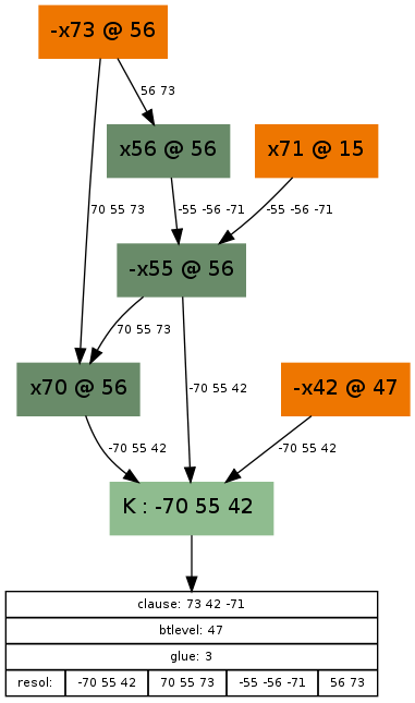
Our first implication graph had a clause “-70 55 42” (light green box) that caused a conflict — that is to say, somehow the variable setting {x70=TRUE, x55=FALSE, x42=FALSE} was set, the SAT solver realised that this is wrong, and something has to be done. Let’s look at what lead here! Guesses are coloured orange here, so it seems we made the following guesses during our SAT solving: x71=TRUE, x73 = FALSE, x42=FALSE. Now, we could just say, oh, well, setting x73 to FALSE was a dumb idea, just reverse that guess, and be done with it. That’s the easy (and the fast) way, but we are less lazy than that and we want to understand the reasons. So we do something called the conflict analysis to find something called an asserting clause that will not only let us reverse the guess x73=FALSE, but will also give the SAT solver a reason why that is a necessary assignment given its previous guesses and their consequences.

Consequences in the graph are coloured dark green, and there are exactly 3 of them: x70=TRUE, x55=FALSE and x56=TRUE. Each of these is a consequence of a clause that is in the SAT solver, marked on the edge(s) leading to it. For example, x56 is set to TRUE, because of the guess x73=FALSE and the clause “x56 V x73” marked on the edge leading to x56. A consequence that has one edge leading to it was propagated by a 2-long clause, a consequence that has 2 edges leading to it was propagated by a 3-long clause (e.g. consequence “x70=TRUE”, propagated by “x70 V x55 V x73”), etc. Okay, so how do we get to the reason? Well, we start out with the conflict, the clause “-x70 V x55 V x42” (at the bottom), and we do resolutions with this clause, going bottom up. We do as many resolutions as needed to reach the first UIP (also called “articulation vertex” or “dominator”), which is a unique point on the graph through which all paths go through from the highest decision level guess, in this case x73=FALSE, at decision level 56 (noted with a @56). If you take a look, the paths from x73=FALSE diverge from the very first point onwards, and there is no single point where they converge again. This means that the (first and only) dominator will be x73=FALSE itself, and we have to resolve with all clauses on the path:

  1. Start with clause “-x70 V x55 V x42”
  2. Resolve with clause “x70 V x55 V x73”
  3. Resolve with clause “-x55 V-x56 V -x71”
  4. Resolve with clause “x56 V x73”

This list is noted on the bottommost box’s lowest entry. When we resolve with these clauses, we are actually doing cuts on the graph, like this:

My drawing capabilities aren’t exactly great, but you can see that the cuts are successively higher and higher, until we reach the cut that has on its outer part the literals -x73, x71 and -x42. Unsurprisingly, exactly the inverse of these literals are what make up the final conflict clause. Now, if we unroll the implications until decision level 47 (but not the guess x42=FALSE), then with this clause added, variable x73 will propagate to TRUE automatically, essentially reversing the wrong guess — but also giving a reason why it needs to be reversed.

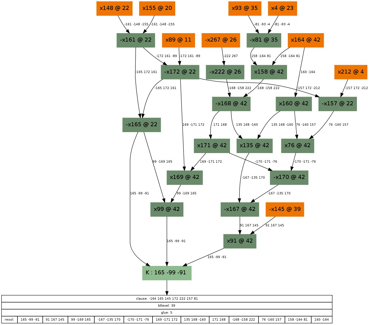
If you enjoyed the previous graph, here is another to entertain you further:

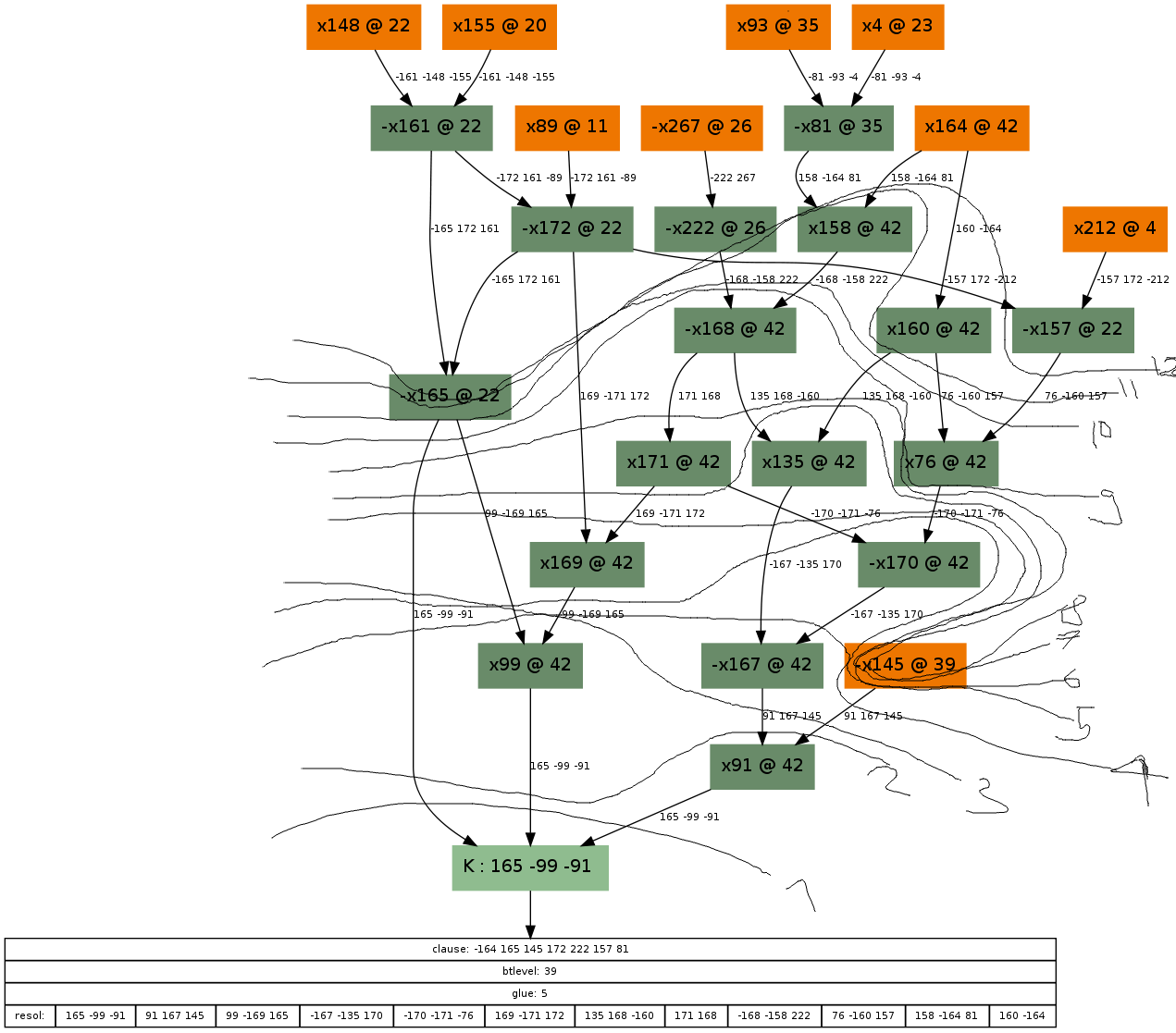
And its corresponding, not too obvious solution:

Note that I was too lazy to draw cuts 10, 11 and 12 around the assignment x145=FALSE (at decision level 39). The UIP in this case is again at the decision variable, x164. If you are still interested, here are some other examples:

PS: Thanks to George Katsirelos for his help understanding this (disclaimer: all faults belong to me alone).