All posts by msoos

ANF to CNF conversion

Algebraic Normal Form, or simply ANF, is the form used to describe cryptographic functions. It looks like this:
a*b \oplus b*c \oplus b \oplus d = 0\\b*c \oplus c \oplus a = 0\\\ldots
Where a,\ldots d are binary variables, the \oplus sign is binary XOR, and the * sign is binary AND. Every item that is connected with the XOR-s is called a monomial, and its degree is the number of independent variables inside it. So, a*b is a 2-degree monomial in the first equation, and c is a 1-degree monomial in the second equation.

An important problem in SAT is to translate an ANF into the input of SAT solvers, Conjunctive Normal Form, or simply CNF. A CNF formula looks like this:
a \vee b \vee c = 1\\a \vee \neg d = 1\\\ldots
Where again a,\ldots d are binary variables, the \vee sign is the binary OR, and the \neg sign is the binary NOT (i.e. inverse).

The scientific reference paper

The most quoted article about ANF-to-CNF translation is that by Courtois and Bard, which advocates for the following translation process:

  1. Introduce internal variables for every monomial of degree larger than 1
  2. Describe the equations as large XORs using the recently introduced variables

The example problem in CNF

According to the original method, the equations presented above are first translated to the following form:
v1 = a*b\\v2 = b*c\\v1 \oplus v2 \oplus b \oplus d = 0\\v2 \oplus c \oplus a = 0

Where v1, v2 are fresh binary variables. Then, each of the above equations are translated to CNF. The internal variables are translated as such:

  1. Translation of v1 = a*b:
    v1 \vee \neg a \vee \neg b = 1\\\neg v1 \vee a = 1\\\neg 1 \vee b = 1
  2. Translation of v2 = b*c
    v2 \vee \neg b \vee \neg c = 1\\\neg v2 \vee b = 1\\\neg v2 \vee c = 1
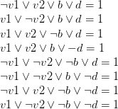
  3. Translation of v1 + v2 + b + d = 0:
    \neg v1 \vee v2 \vee b \vee d = 1\\v1 \vee \neg v2 \vee b \vee d = 1\\v1 \vee v2 \vee \neg b \vee d = 1\\v1 \vee v2 \vee b \vee -d = 1\\\neg v1 \vee \neg v2 \vee \neg b \vee d = 1\\\neg v1 \vee \neg v2 \vee b \vee \neg d = 1\\\neg v1 \vee v2 \vee \neg b \vee \neg d = 1\\v1 \vee \neg v2 \vee \neg b \vee \neg d = 1
  4. Translation of v2 + c + a = 0 :
    v2 \vee c \vee \neg a = 1\\v2 \vee \neg c \vee a = 1\\\neg v2 \vee c \vee a = 1\\\neg v2 \vee \neg c \vee \neg a = 1

We are now done. The final CNF file is this. This final CNF  has a small header, and some  fluffs have been removed: variables are not named, but referred to with a number, and the = true-s have been replaced with a line-ending 0.

As you can imagine, there are many ways to enhance this process. I have written a set of them down in this paper. The set of improvements in a nutshell are the following:

  1. If a variable’s value is given, (e.g. a = true), first substitute this value in the ANF, and transcribe the resulting ANF to CNF.
  2. If there are two monomials, such as: a*b + b in an equation, make a non-standard monomial (-a)*b from the two, and transcribe this to CNF. Since the CNF can use negations, this reduces the size of the resulting CNF
  3. If the ANF can be described using Karnaugh maps shorter than with the method presented above, use that translation method.

An automated way

I just got a nice script to perform step (1) from Martin Albrecht, one of the developers of Sage:

sage: B = BooleanPolynomialRing(4500,'x')
sage: L = [B.random_element(degree=2,terms=10) 
      for _ in range(4000)]
sage: s = [B.gen(i) + GF(2).random_element() 
      for i in range(1000)]
sage: %time F = 
      mq.MPolynomialSystem(L+s).
      eliminate_linear_variables(maxlength=1)
CPU time: 1.03 s,  Wall time: 1.11 s

In this code, Martin generates a boolean system of equations with 4500 variables, with 4000 random equations each with randomly selected monomials of degree 2 and of XOR size 10. Then, he sets 1000 random variables to a random value (true or false), and finally, he substitutes the assigned values, and simplifies the system. If you think this is a trivial issue, alas, it is not. Both Maple and Sage take hours to perform it if using the standard eval function. The function above uses a variation of the ElimLin algorithm from the Courtois-Bard paper to do this efficiently.

How to bit-stuff pointers

In my last post I have described a small problem I had regarding a C++ union that had to store a pointer and a value at the same time, plus an indicator that told us which of the two was active:

class WhatLeadHere {
public:
    bool wasPointer;
    union{Clause* pointer; uint32_t lit;};
};

Martin Maurer has wrote this enlightening email regarding this:

The Clause * pointer is [..] located at least on a 4 byte boundary (at least when not forced by e.g. #pragma). If it is not at least on a 4 byte boundary, CPU must (at least some of them) do two accesses: one lower DWORD, one upper DWORD, and merge both together, which reduces speed.

So the lower two bits are always zero :-) Why not move the “wasPointer” to lower two bits (i think you need only one, have one spare bit). Of course before accessing the “pointer” (Clause *), you must “and” the two lower bits back to zero.

He is perfectly right: the pointer will never be zero on the least significant bit (LSB), so setting that to “1” can be used as an indicator. This is a form of bit-stuffing. To check if it’s a pointer or a literal the following function can be used:

const bool WhatLeadHere::wasPointer() const
{
   return (lit&1);
}

As for storing lit, we need to right-shift it by one and set the LSB to 1. When lit is needed, we left-shift it to get back the original value. This is not a problem, since variables in SAT never use out the 32-bit space: there are rarely more than 10 million variables, so right-shifting this value will not lead to information loss.

Propagating binary clauses

Binary clauses are somewhat special. They are clauses that look like:

-v1 or v20 = true
-v1 or v21 = true

which basically mean: if v1 is TRUE, then both v20 and v21 must be TRUE. We put these clauses into a special datastructure, that looks like this:

watchlist[-v1] = v20,v21, ...

This makes us all very happy, since this datastructure is very simple: just literals (negated or non-negated variables) one after the other, in a very trivial list. This makes the whole thing very compact, and very efficient.

The problem with such a list is that when v1 is indeed set to TRUE, then when we set the variables (e.g. v20,v21), we must record what set these variables to their new values. What usually is done is to simply record the pointer to the clause that does this. However, in the above datastructure, there are no clause pointers. The datastructure for GLUCOSE contained these pointers. I have lately been experimenting with removing these pointers. The tricky part is to update the conflict generation routine that examines the clauses and decisions that lead to a conflict. This routine must now automatically recognise that these binary clauses are special, and they are only 2-long: one part of them is the variable that got set, and the other part is the variable that set it. These two informations are available: watchlist[-v1] immediately tells us that literal -v1 set the variable, and the variable that got set is always known.

Armed with this logic, one would think that moving towards this all-new no-clause-pointers heaven is the way to go. However, apparently, this might not be so. This is quite astonishing, given that doing things without pointers should mean less cache-misses (since pointers are less likely to be resolved during conflict analysis). I consistently get worse speeds, though. I am guessing that the problem lies with the datastructure I use to store the information stating what lead to the setting of the variable. I use a very simple struct:

struct WhatLeadHere {
    bool wasPointer;
    union{Clause* pointer; Lit lit;};
};

where wasPointer is TRUE if a non-binary clause lead here (and we store the pointer), and FALSE if it was a binary clause (and we store the other literal). The union takes care of the rest: pointer is valid when wasPointer is TRUE and lit is valid when wasPointer is FALSE.

What is apparent in this datastructure is the following: we now store a 32/64 bit pointer plus we store a boolean. Right, so 42/72 bits of data? No. Data alignment in C++ means, that this datastructure will be aligned according to its largest member, so it will be aligned to 32/64-bit boundaries: this datastructure takes 128/64 bits to store on 32 and 64 bit architectures, respectively. Oops, we just doubled our demand of data writes!

There are some remedies, of course. We can simply pack:

#pragma pack(push)
#pragma pack(1)
struct WhatLeadHere {
    bool wasPointer;
    union{Clause* pointer; Lit lit;};
};
#pragma pack(pop)

which removes the memory burden of aligning to maximum size, and the actual size will really be 42/72 bits. But this reaises the overhead of accessing data inside this structure. Furthermore, I have been using a 32-bit mini-pointer on 64-bit architectures, which is a big hack, so it crumbles as soon as something as complicated as this comes up: so I am left with writing 72 bits instead of 32. This probably leads to the slowdowns. Oh well, I have got to work harder…

EDITED TO ADD: Next up, I will talk about some new ideas that let me solve 217 problems from the 2009 SAT Race within the original time limit. Remember that last year the best solver only solved 204.

Optimisations, take two

I have talked about optimisations before and I mentioned that there are a few left to describe. In this post I will talk about two of them.

The first optimisation I would like to talk about concerns compilation flags. Somehow, everyone seems obsessed with them, like if they could somehow make a slow program fast. Alas, this is not the case. Firstly, and this is quite funny: the gcc flag “-O3” usually turns on all extra flags that people tend to give. One should really ponder upon this when looking at desperate attempts to speed up code. However, there is exactly one flag-combo that is very-very useful besides “-O3”: it’s “-fprofile-generate” and “-fprofile-use”. To understand why these are useful, we must first understand that one of the challenges faced by an optimising compiler is to try to guess how many times a loop will be executed,and how many times a branch will be taken. Given a good set of guesses, the loop can be unwound (or not) and the branches can be taken by default (or not). If compiled with “-fprofile-generate”, the program generates such information on-the-fly, which later can be used by “-fprofile-use”. The speedup achieved with such an approach in the realms of DPLL-based SAT solvers is relatively high, in the order of ~5-10%. I believe many SAT solvers’ binaries don’t use this trick, even though it’s cheap to use. I personally compile with “-fprofile-generate”, then run an example problem like UTI-20-10p1 on it, and then recompile with “-fprofile-use”. An important aspect, by the way, is to execute your problem with a very typical scenario: strange or non-normal scenarios will produce spurious branching and loop data which will actually slow down the program most of the time instead of speeding it up.

The second optimisation I would like to talk about concerns cache usage. Modern processors are extremely fast, to the point that many times what really limits the processor is no longer the ability to execute the code on the data, but to actually get the data that the code needs. This problem is usually alleviated through spatial and temporal data locality that is, that data most likely needed next is usually physically close to the one that we just accessed. However, in DPLL-based SAT solvers, the main function, propagate() goes through a list of pointers, accessing the data where each pointer points to. In other words, the CPU will fetch the next pointer in the background, but will not fetch where that pointer points to — simply because it doesn’t know it’s a pointer. So, how could we alleviate this problem? Well, by telling the CPU that the next piece of information that will be needed is where the next pointer points to. Like this:

for (i = 0; i < pointers.size();  i++) {
    if (i+1 < pointers.size())
        __builtin_prefetch(pointers[i+1]);
    treat_data(*pointers[i]);
}

where pointers is a vector of pointers that must each be treated. The function __builtin_prefetch() calls an assembly instruction that non-blockingly fetches the data pointed to into the Level 1 cache of the processor. This/these instruction(s) are not implemented in all CPUs, but many x86 and all AMD64 architectures have them. Essentially, while we are dealing with data where pointers[i] points at, we fetch the data where pointers[i+1] points at, in parallel. Interleaving the fetching of next data with the treatment of current data helps us do more things in less time, speeding up the program. Interestingly, since prefetching the data does not alter the flow of the program in any way, omitting the prefetch call does not alter the results of the program at all: it just makes it run slower. In CryptoMiniSat I use this optimisation, and it seems to speed up the solving by a couple of percentages, maybe 5-8%. The amount of time you will save on this depends on the locality and size of the information your pointers are pointing to. If they are very small, e.g. 2-3MB in total and are close to each other, then the CPU will fetch these after the first couple of pointers have been dereferenced, so there is no need to do explicit prefetching. But if the data you are dealing with is much larger, which is often the case with SAT solvers, then such explicit pre-fetching can save quite some time.

The Obvious Child

The new CryptoMiniSat 2.5.1, codenamed “The Obvious Child” has been released. It’s very close to the system that has been sent into the SAT Race’10. This version of CryptoMS is much better than any versions before: I finally corrected a lot of bugs that went into the 2.4.x series, and added new features to treat binary clauses.

The release name is the song title by Paul Simon. I am a fan of the 60’s for many reasons. It was the time when Laing wrote his first books, empathy was first scientifically demonstrated for animals, the days of I have a dream, the landing on the moon, and the take-off of Simon&Garfunkel.; Some interesting times, shall we say.

I probably will be working less on CryptoMiniSat from now on, instead concentrating on other things that I must do, such as publishing research papers on subjects that interest the scientific community. I will also be trying to play out in my mind how CryptoMiniSat will fare in the SAT Race. Of course I am hoping for the best, but I worked on the program for a mere 8 months, alone. Comparing this to some experts working on their solvers for multiple years in groups of 2-3, I really have no chance of winning. However, I am optimistic, as always: maybe I will get some good position in the rankings :)