All posts by msoos

On SAT/SMT Model Counting

I have recently had a few discussions with people who wanted to do some form of model counting, and I decided to put my thoughts about this problem into a single blog post, hopefully bringing some light to this area. Firstly, when talking about model counting, it’s very important to think through what one actually needs to achieve. When people talk about a model, they often mean a solution to a problem, described as a set of constraints over either purely boolean variables (so-called propositional model counting) expressed in so-called CNF, or over higher-level constraints, often expressed in SMT-LIB format.

Let’s look at a CNF example:

c this is a comment
c below line means there are 5 boolean variables and 2 constraints
p cnf 5 2
1 -2 0
1 -2 3 0

The above CNF has 5 boolean variables and 2 constraints: “v1 or (not v2) = true”, and “v1 or (not v2) or v3 = true”. In this case, if “v1 or (not v2) = true” is satisfied, the other constraint is also satisfied. So we effectively only have to satisfy the “v1 or -v2” constraint. There are 3 solutions over the variables v1 and v2 to this constraint: (1, 0), (1, 1), and (0,0). For variables v3, v4, and v5 we can choose anything. So there are a total of 3*2^3 = 24 solutions to this CNF.

Let’s look at an SMT problem:

(set-logic QF_BV) ; Set the logic to Quantifier-Free BitVectors
(declare-fun bv () (_ BitVec 8)) ; Declare an 8-bit value
(assert (not (= bv #x00))) ; Assert that 'bv' is not equal to zero

In this SMT-LIB problem, we declared that the logic we will be using is the so-called quantifier-free bitvector logic, which basically gives you access to fixed-width variables such as uint8_t, and of course all the logical and fixed-bit bitwector operators such as modulo addition, division, subtraction, etc. In this particular case, we declared an 8-bit variable and banned it from being 0, so this problem has 2^8-1 solutions, i.e. 255.

Whichever format is being used, “counting” of solutions is something that may sound trivial (it’s just a number!), but once we get a bit more fiddly, it turns out that we can do many things that are actually easier, or even harder, than just counting, even though they sound very close to, or are even synonymous with, counting :

  • Figuring out if there is at least one solution. This is more appropriately called satisfiability checking. This is significantly easier than any notion of counting listed below. However, even this can be challenging. Typically, in the SMT/SAT competition, this is the so-called SMT single query track or the SAT competition Main Track. All SAT and SMT solvers such as kissat or cvc5 can run this kind of task.
  • Next up in complexity is to figure out if there is exactly one solution. This is actually very close to satisfiability checking, and requires only two so-called “incremental calls” to the SMT/SAT solver. I have seen this question pop up a lot in zero-knowledge (ZK) circuit correctness. What is needed is to run the query as per the above, but then add a constraint that bans the solution that is output by the solver, and ask the system to be solved again. If the solver outputs UNSAT, i.e. unsatisfiable, then we know there are no more solutions, and we are happy with the result. If not, it gives us another solution, which is a witness that there are at least two solutions. These queries are answered by so-called incremental SMT solvers (SMT competition track here), or incremental SAT solvers (incremental SAT competition track here). Almost all SAT and SMT solvers can work incrementally, for example cvc5 or z3. Most SAT solvers work incrementally, too, but e.g. kissat does not, and you need to use CaDiCaL instead.
  • Next up in complexity is to approximately count the solutions. Here, we are not interested that there are exactly, say, 87231214 solutions, instead, we are happy to know that there are approx 2^26 solutions. This is often good enough, in case one wants to e.g. figure out probabilities. There are very few such systems available, for SMT there is csb, and for SAT there is ApproxMC. For the special case of approximate DNF counting, I’d recommend pepin.
  • Next up in the complexity is exactly counting the solutions. Here, we want to know how many solutions there are, exactly, and we really-really need the exact number. There are few solutions to doing this over SMT, but doing this over SAT is quite developed. For SMT, I would recommend following the csb approach, and running Ganak on the blasted SAT formula instead of ApproxMC, and for SAT, there is the annual model counting competition, where Ganak won every single category this year, so I’d recommend Ganak.
  • Next up is model enumeration where it’s not enough to count the solutions, but we need a way to compactly represent and store them all. This of course requires quite a bit of disk space, as there could be e.g. 2^100 solutions, and representing them all, even in a very compact format with lots of smart ideas can take a lot of space — but not necessarily exponential amount. Currently, there is no such system for SMT, and my understanding is that only the d4 model counter can do this on SAT/CNF problems, thanks to its proof checking system, in part thanks to Randal Byrant. Once Ganak can output a proof, it will also be able to do this.

All in all, there is a very large gap between “find if there is exactly one solution” and “enumerate all solutions” — even though I have seen these two notions being mixed up a few times. The first might take only a few seconds to solve, while the other might not even be feasible, because compactly representing all solutions may be too expensive in terms of space (and that’s not even discussing time).

One aspect to keep in mind is that often, one does not need all solutions. For example, if one only wants to find a good set of example solutions, then it is possible to use uniform-like samplers, that give a “somewhat uniform” set of example solutions from the solution space (without guarantees of uniformity). A good tool for this is cmsgen for CNF/SAT problems. If one needs a guaranteed uniform set of samples (to be exact, a probabilistically approximately uniform sample), then unigen is the way to go. Obviously, it’s quite easy to find a uniform sample once we have an enumeration of all solutions — simply pick a random one from the whole set — but that’s way more expensive than running unigen.

While all of the above is about counting, it’s often the case that one wants to optimize for something within the solution space. Basically, we have some kind of objective function that we want to optimize for (e.g. maximize profit, minimize loss) , and so we are looking for a solution that maximizes/minimizes some property. Of course, once we have done model enumeration, it’s quite easy to do this — simply run the objective function on all solutions, and pick the best! But that’s really hard. Instead, one can formulate the problem as a so-called MaxSAT or an SMT problem with an objective function. These systems run some really smart algorithms to significantly cut down search time, and even often keep a “best so far” solution around, so we can early-abort them and still get some kind of “best so far” solution.

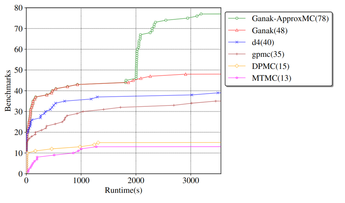
All in all, it’s extremely important to figure out what one actually needs, because there are vast gaps in complexity between the problems (and corresponding algorithms) above. Even between something like approximate and exact counting, the gap is gigantic, as there are huge swaths of problems that are almost trivial to count approximately, but essentially impossible to exactly count with current technology:

Here, the green line is a tool that changes its behaviour from exact to approximate model counting after 1800 seconds of solving, and the number of solved instances jumps significantly. Notice that the red line, the original system it runs for 1800s, is the best in class here, by a wide margin, and still the approximate counting that Ganak+ApprocMC switches into shows a massive difference.

Our tools for solving, counting and sampling

This post is just a bit of a recap of what we have developed over the years as part of our toolset of SAT solvers, counters, and samplers. Many of these tools depend on each other, and have taken greatly from other tools, papers, and ideas. These dependencies are too long to list here, but the list is long, probably starting somewhere around the Greek period, and goes all the way to recent work such as SharpSAT-td or B+E. My personal work stretches back to the beginning of CryptoMiniSat in 2009, and the last addition to our list is Pepin.

Overview

Firstly when I say “we” I loosely refer to the work of my colleagues and myself, often but not always part of the research group lead by Prof Kuldeep Meel. Secondly, almost all these tools depend on CryptoMiniSat, a SAT solver that I have been writing since around 2009. This is because most of these tools use DIMACS CNF as the input format and/or make use of a SAT solver, and CryptoMiniSat is excellent at reading, transforming , and solving CNFs. Thirdly, many of these tools have python interface, some connected to PySAT. Finally, all these tools are maintained by me personally, and all have a static Linux executable as part of their release, but many have a MacOS binary, and some even a Windows binary. All of them build with open source toolchains using open source libraries, and all of them are either MIT licensed or GPL licensed. There are no stale issues in their respective GitHub repositories, and most of them are fuzzed.

CryptoMiniSat

CryptoMiniSat (research paper) our SAT solver that can solve and pre- and inprocess CNFs. It is currently approx 30k+ lines of code, with a large amount of codebase dedicated to CNF transformations, which are also called “inprocessing” steps. These transformations are accessible to the outside via an API that many of the other tools take advantage of. CryptoMiniSat used to be a state-of-the-art SAT solver, and while it’s not too shabby even now, it hasn’t had the chance to shine at a SAT competition since 2020, when it came 3rd place. It’s hard to keep SAT solver competitive, there are many aspects to such an endeavor, but mostly it’s energy and time, some of which I have lately redirected into other projects, see below. Nevertheless, it’s a cornerstone of many of our tools, and e.g. large portions of ApproxMC and Arjun are in fact implemented in CryptoMiniSat, so that improvement in one tool can benefit all other tools.

Arjun

Arjun (research paper) is our tool to make CNFs easier to count with ApproxMC, our approximate counter. Arjun takes a CNF with or without a projection set, and computes a small projection set for it. What this means is that if say the question was: “How many solutions does this CNF has if we only count solutions to be distinct over variables v4, v5, and v6?”, Arjun can compute that in fact it’s sufficient to e.g. compute the solutions over variables v4 and v5, and that will be the same as the solutions over v4, v5, and v6. This can make a huge difference for large CNFs where e.g. the original projection set can be 100k variables, but Arjun can compute a projection set sometimes as small as a few hundred. Hence, Arjun is used as a preprocessor for our model counters ApproxMC and GANAK.

ApproxMC

ApproxMC (research paper) is our probabilistically approximate model counter for CNFs. This means that when e.g. ApproxMC gives a result, it gives it in a form of “The model count is between 0.9*M and 1.1*M, with a probability of 99%, and with a probability of 1%, it can be any value”. Which is very often enough for most cases of counting, and is much easier to compute than an exact count. It counts by basically halfing the solution space K times and then counts the remaining number of solutions. Then, the count is estimated to be 2^(how many times we halved)*(how many solutions remained). This halfing is done using XOR constraints, which CryptoMiniSat is very efficient at. In fact, no other state-of-the-art SAT solver can currently perform XOR reasoning other than CryptoMiniSat.

UniGen

UniGen (research paper) is an approximate probabilistic uniform sample generator for CNFs. Basically, it generates samples that are probabilistically approximately uniform. This can be hepful for example if you want to generate test cases for a problem, and you need the samples to be almost uniform. It uses ApproxMC to first count and then the same idea as ApproxMC to sample: add as many XORs as needed to half the solution space, and then take K random elements from the remaining (small) set of solutions. These will be the samples returned. Notice that UniGen depends on ApproxMC for counting, Arjun for projection minimization, and CryptoMiniSat for the heavy-lifting of solution/UNSAT finding.

GANAK

GANAK (research paper, binary) is our probabilistic exact model counter. In other words, it returns a solution such as “This CNF has 847365 solutions, with a probability of 99.99%, and with 0.01% probability, any other value”. GANAK is based on SharpSAT and some parts of SharpSAT-td and GPMC. In its currently released form, it is in its infancy, and while usable, it needs e.g. Arjun to be ran on the CNF before, and while competitive, its ease-of-use could be improved. Vast improvements are in the works, though, and hopefully things will be better for the next Model Counting Competition.

CMSGen

CMSGen (research paper) is our fast, weighted, uniform-like sampler, which means it tries to give uniform samples the best it can, but it provides no guarantees for its correctness. While it provides no guarantees, it is surprisingly good at generating uniform samples. While these samples cannot be trusted in scenarios where the samples must be uniform, they are very effective in scenarios where a less-than-uniform sample will only degrade the performance of a system. For example, they are great at refining machine learning models, where the samples are taken uniformly at random from the area of input where the ML model performs poorly, to further train (i.e. refine) the model on inputs where it is performing poorly. Here, if the sample is not uniform, it will only slow down the learning, but not make it incorrect. However, generating provably uniform samples in such scenarios may be prohibitively expensive. CMSGen is derived from CryptoMiniSat, but does not import it as a library.

Bosphorus

Bosphorus (research paper) is our ANF solver, where ANF stands for Algebraic Normal Form. It’s a format used widely in cryptography to describe constraints over a finite field via multivariate polynomials over a the field of GF(2). Essentially, it’s equations such as “a XOR b XOR (b AND c) XOR true = false” where a,b,c are booleans. These allow some problems to be expressed in a very compact way and solving them can often be tantamount to breaking a cryptographic primitive such as a symmetric cipher. Bosphorus takes such a set of polynomials as input and either tries to simplify them via a set of inprocessing steps and SAT solving, and/or tries to solve them via translation to a SAT problem. It can output an equivalent CNF, too, that can e.g. be counted via GANAK, which will give the count of solutions to the original ANF. In this sense, Bosphorus is a bridge from ANF into our set of CNF tools above, allowing cryptographers to make use of the wide array of tools we have developed for solving, counting, and sampling CNFs.

Pepin

Pepin (research paper) is our probabilistically approximate DNF counter. DNF is basically the reverse of CNF — it’s trivial to ascertain if there is a solution, but it’s very hard to know if all solutions are present. However, it is actually extremely fast to probabilistically approximate how many solutions a DNF has. Pepin does exactly that. It’s one of the very few tools we have that doesn’t depend on CryptoMiniSat, as it deals with DNFs, and not CNFs. It basically blows all other such approximate counters out of the water, and of course its speed is basically incomparable to that of exact counters. If you need to count a DNF formula, and you don’t need an exact result, Pepin is a great tool of choice.

Conclusions

My personal philosophy has been that if a tool is not easily accessible (e.g. having to email the authors) and has no support, it essentially doesn’t exist. Hence, I try my best to keep the tools I feel responsible for accessible and well-supported. In fact, this runs so deep, that e.g. CryptoMiniSat uses the symmetry breaking tool BreakID, and so I made that tool into a robust library, which is now being packaged by Fedora, because it’s needed by CryptoMiniSat. In other words, I am pulling other people’s tools into the “maintained and supported” list of projects that I work with, because I want to make use of them (e.g. BreakID now builds on Linux, MacOS, and Windows). I did the same with e.g. the Louvain Community library, which had a few oddities/issues I wanted to fix.

Another oddity of mine is that I try my best to make our tools make sense to the user, work as intended, give meaningful (error) messages, and good help pages. For example, none of the tools I develop call subprocesses that make it hard to stop a computation, and none use a random number seed that can lead to reproducibility issues. While I am aware that working tools are sometimes less respected than a highly cited research paper, and so in some sense I am investing my time in a slightly suboptimal way, I still feel obliged to make sure the tax money spent on my academic salary gives something tangible back to the people who pay for it.

The Inprocessing API of CryptoMiniSat

Many modern SAT solvers do a lot of what’s called inprocessing. These steps simplify the CNF into something that is easier to solve. In the compiler world, these are called rewritngs since the effectively rewrite (parts of) the formula to something else that retain certain properties, such as satisfiability. One of the most successful such rewrite rules for CNF is Bounded Variable Elimination (BVE, classic paper here), but there are many others. These rewrites are usually done by modern SAT solvers in a particular order that was found to be working well for their particular use-case, but they are not normally accessible from the outside.

Sometimes one wants to use these rewrite rules for something other than just solving the instance via the SAT solver. One such use-case is to use these rewrite rules to simplify the CNF in order to count the solution to it. In this scenario, the user wants to rewrite the CNF in a very particular way, and then extract the simplified CNF. Other use-cases are easy to imagine, such as e.g. MaxSAT, core counting, etc. Over the years, CryptoMiniSat has evolved such a rewrite capability. It is possible to tell CryptoMiniSat to simplify the formula exactly how the user wants the solver to be satisfied and then extract the simplified formula.

Example Use-Case

Let’s say we have a CNF that we want to simplify:

p cnf 4 2
1 2 3 4 0
1 2 3 0

In this CNF, 1 2 3 4 0 is not needed, because it is subsumed by the clause 1 2 3 0. You can run subsumption using CryptoMiniSat this way:

#include "cryptominsat5/cryptominisat.h"
#include <vector>
#include <cmath>
#include <iostream>

using namespace CMSat;
using namespace std;
#define lit(a) Lit(std::abs(a)-1, a<0)

int main() {
  Solver s;
  vector<Lit> cl;
  s.add_new_vars(4);

  cl = vector<Lit>{lit(1), lit(2), lit(3), lit(4)};
  s.add_clause(cl);
  cl = vector<Lit>{lit(1), lit(2), lit(3)};
  s.add_clause(cl);
  
  s.simplify(NULL, "occ-backw-sub");
  s.start_getting_clauses();
  while(s.get_next_clause(cl) {
    for(const auto l: cl) cout << l << " ";
    cout << endl;
  }
  s.end_getting_clauses()
  
  return 0;
}

This code runs the inprocessing system occ-backw-sub, which stands for backwards subsumption using occurrence lists. The input CNF can be anything, and the output CNF is the simplified CNF. This sounds like quite a lot of code for simple subsumption, but this does a lot of things under the hood for things to be fast, and it is a lot more capable than just doing subsumption.

Notice that the first argument we passed to simplify() is NULL. This means we don’t care about any variables being preserved — any variable can (and will) be eliminated if occ-bve is called. In case some variables are important to you not to be eliminated, you can create a vector of them and pass the pointer here. If you have called the renumber API, then you can get the set of variables you had via clean_sampl_and_get_empties(). The numbering will not be preserved, but their set will be the same, though not necessarily the same size. This is because some variables may have been set, or some variables may be equivalent to other variables in the same set. You can get the variables that have been set via get_zero_assigned_lits().

Supported Inprocessing Steps

Currently, the following set of inprocessing steps are supported:

API nameInprocessing performed
occ-backw-subBackwards subsumption using occurence lists
occ-backw-sub-strBackwards subsumption and strengthening using occurence lists
occ-bceBlocked clause elimination (paper)
occ-ternary-resTernary resolution (paper)
occ-lit-remLiteral removal via strengthening
occ-cl-rem-with-orgatesOR-gate based clause removal (unpublished work, re-discovered by others)
occ-rem-with-orgatesOR-gate based literal removal
occ-bveBounded variable elimination (paper)
occ-bve-emptyBounded variable elimination of empty resolvents only
intree-probeProbe using in-tree probing, also do hyper-binary resolution and transitive reduction (paper). Also does hyper-binary resoution & transitive reduction
full-probeProbe each literal individually (slow compared to intree-probe)
backboneBackbone simplification (cadiback paper)
sub-implSubsume with binary clauses with binary clauses (fast)
sub-str-cls-with-binSubsume and strengthen long clauses with binary clauses (fast)
sub-cls-with-binSubsume long clauses with binary clauses (fast)
distill-binsDistill binary clauses
distill-clsDistill long clauses (distillation paper)
distill-cls-onlyremDistill long clauses, but only remove clauses, don’t shorten them. Useful if you want to make sure BVE can run at full blast after this step.
clean-clsClean clauses of set literals, and delete satisfied clauses
must-renumberRenumber variables to start from 0, in case some have been set to TRUE/FALSE or removed due to equivalent literal replacement.
must-scc-vreplPerform strongly connected component analysis and perform equivalent literal replacement.
oracle-vivifyVivify clauses using the Oracle tool by Korhonen and Jarvisalo (paper). Slow but very effective.
oracle-vivif-sparsifyVivify & sparsify clauses using the Oracle tool by Korhonen and Jarvisalo. Slow but very effective.

Convenience Features Under the Hood

The steps above do more than what they say on the label. For example, the ones that start with occ build an occurrence list and use it for the next simplification stop if it also starts with occ. They also all make sure that memory limits and time limits are adhered to. The timeout multiplier can be changed via set_timeout_all_calls(double multiplier). The time limits are entirely reproducible, there is no actual seconds, it’s all about an abstract “tick” that is ticking. This means that all bugs in your code are always reproducible. This helps immensely with debugging — no more frustrating Heisenbugs. You can check the cryptominisat.h file for all the different individual timeouts and memouts you can set.

Under the hood you also get a lot of tricks implemented by default. You don’t have to worry about e.g. strengthening running out of control, it will terminate in reasonable amount of ticks, even if that means it will not run to completion. And the next time you run it, it will start at a different point. This makes a big difference in case you actually want your tool to be usable, rather than just “publish and forget”. In many cases, simplification only makes things somewhat faster, and you want to stop performing the simplification after some time, but you also want your users to be able to report bugs and anomalies. If the system didn’t have timeouts, you’d run the risk of the simplifier running way too long, even though the actual solving would have taken very little time. And if the timeout was measured in seconds, you’d run the risk of a bug being reported but being irreproducible, because the exact moment the timeout hit for the bug to occur would be irreproducible.

Making the Best of it All

This system is just an API — it doesn’t do much on its own. You need to play with it, and creatively compose simplifications. If you take a look at cryptominisat.h, it already has a cool trick, where it moves the simplified CNF from an existing solver to a new, clean solver through the API, called copy_simp_solver_to_solver(). It is also used extensively in Arjun, our CNF simplifier for counting. There, you can find the function that controls CryptoMiniSat from the outside to simplify the CNF in the exact way needed. It may be worthwhile reading through that function if you want to control CryptoMiniSat via this API.

The simplify() API can give you the redundant clauses, too (useful if you e.g. did ternary or hyper-binary resolution), and can give you the non-renumbered CNF as well — check out the full API in cryptominisat.h, or the Arjun code. Basically, there is a red and a simplified parameter you can pass to this function.

Perhaps I’ll expose some of this API via the Python interface, if there is some interest for it. I think it’s quite powerful and could help people who use CNFs in other scenarios, such as MaxSAT solving, core counting, core minimization, etc.

Closing Thoughts

I think there is currently a lack of tooling to perform the already well-known and well-documented pre- and inprocessing steps that many SAT solvers implement internally, but don’t expose externally. This API is supposed to fill that gap. Although it’s a bit rough on the edges sometimes, hopefully it’s something that will inspire others to either use this API to build cool stuff, or to improve the API so others can build even cooler stuff. While it may sound trivial to re-implement e.g. BVE, once you start going into the weeds of it (e.g. dealing with the special case of detecting ITE, OR & AND gates’ and their lower resolvent counts, or doing it incrementally with some leeway to allow clause number increase), it gets pretty complicated. This API is meant to alleviate this stress, so researchers and enthusiasts can build their own simplifier given a set of working and tested “LEGO bricks”.

Pepin, our Probabilistic Approximate Volume Counter

Let’s say you are allowed to have cubes in a 3-dimensional space that happens to be binary. In this space, x1, x2, and x3 are the axis, and for example the cube x1=0 is a cube that happens to have 4 points in it: 000, 001, 010, and 011. So far, so good. Now, let’s say we need to calculate the total volume of two cubes in this space. If they don’t intersect, it’s quite easy, we simply add their volumes. But what if they intersect? Now we need to compute their overlap, and subtract it from their sum of volumes. But there is a better way.

Probabilistic Approximate Volume Counting

Our new tool Pepin (code, paper) is based on the probabilistic approximate model counting algorithm by Meel, Vinodchandran, and Chakraborty (paper) that is so simple in principle yet so ingenious that even Donald Knuth got excited about it, recently writing a 15-page note and spending considerable amount of time on the algorithm.

So, what is this algorithm? Well, it’s so simple it’s almost funny. Basically, we keep randomly sampled points from the volume that we currently hold. At every moment we have a representative, evenly sampled set of points from the volume we currently have, and we know the sampling rate. You can think of the “sampling rate” as the approximate volume that each sample represents. So, if at any point we want to know the volume, we calculate number_of_points*(1/sampling_rate) and have the approximate volume. Kinda neat, no? So all we need is a randomly sampled set of points and a corresponding sampling rate. But how do we go about that?

Let’s say we are about to process the first cube (i.e. volume, could be any shape, actually, but cubes are simple). Our sampling rate is 1.0, we have 10 dimensions, and we have a limit of 10 samples in our bag. Let’s say the first cube is:

x1=0

Notice that this cube has 2^9 elements: 0000000000, 0000000001, … 0111111111. But that’s too many elements to hold, we only have space for 10 samples in the bag! We have to drop our sampling rate. The algorithm throws coins for each element in the volume (at first, a coin that has 1.0 probability of heads… funny coin!), and realizes that it won’t fit the sample bag. So it halves the sample rate (to 0.5) and throws the coins again. Realizes it doesn’t fit… halves the sample rate… and eventually will likely end up with a sampling rate of 1/2^6. That sample rate makes sense: it means 2^9/2^6 = 9 samples on average, which fits. Let’s say the algorithm flipped the coins, halved the sampling rate every time, and settled on a sampling rate of 1/2^6, and 9 samples.

Let’s see these samples. For readability, I’ll write the samples as 0110… which means x1=0, x2=1, x3=1, x4=0, etc.

0001011110
0010110110
0010000101
0001101001
0101001011
0011110101
0101101001
0110101100
0000011111

Think of each of these points representing a volume of 2^6. The current estimate of the volume is 9*2^6 = 2^9.17 (instead of 2^9). So far so good. Now a new cube comes in. Let’s say this cube is:

x1=0, x1=1

This is the tricky part. What do we do? The algorithm is extremely simple: we throw away every sample that matches this cube, and then we sample the cube. Let’s throw away everything that matches, i.e. everything that starts with “01”:

0001011110
0010110110
0010000101
0001101001
0011110101
0000011111

Good. Now we sample the cube “x1=0, x1=1” with 1/2^6 probability. Time to take out our weird coin that has a 1/2^6 chance of winning! We toss this coin on every element in the cube, i.e. all 2^8 (since x0=1, x1=1 has 2^8 elements). We should get about 4 heads, but let’s say we got 3. Happens. Now, append these 3 to our neat little sample bag:

0001011110
0010110110
0010000101
0001101001
0011110101
0000011111
0101001011
0101111101
0110000010

Nice. What just happened? Well, we got rid of the elements from the volume we were holding that were contained in the cube that we are processing. Then, we randomly sampled elements from the cube at our given sampling rate. If you think about it, this means that as long as we did everything uniformly at random, we are basically back to where we started. In fact, the 2nd cube could have been anything. It could have been completely outside of our current volume, or it could have partially intersected it. The game is the same. Running out of space? Just throw away each sample with probability half, and half your sampling rate! Here’s a visual representation what we would do in case the two cubes partially intersected:

As the number of samples goes over the limit in our bag, we simply throw away each sample with 0.5 probability, and halve our sampling rate. This allows us to keep a fixed maximum number of samples, regardless of the size of the volume we are holding. For our example, we decided to limit ourselves to 10 samples, and got a pretty good estimate of the volume: 9*2^6 (=~2^9.17) instead of 2^9. One thing of note. This algorithm is not only approximate in the sense that we get something close to the actual solution, like 2^9.17. It’s also probabilistic in the sense that with a low probability, we get a complete garbage value. You can reduce the probability of getting a garbage value in a number of ways, though.

This algorithm is really powerful, because you could approximately count a 100-dimensional volume with thousands of cubes using less than 1MB of memory, and actually be pretty damn accurate, with a very low probability of getting a wrong value. Unsurprisingly, this is exactly what we do in our tool, Pepin.

The Tricks of Pepin

If you think about it, Pepin does nothing but: (1) holds a bunch of samples (2) deals with some large & small numbers (2^10000 is large, and 1/2^100000 is small), and (3) deals with probabilities. For dealing with small & large numbers, we used the GNU MP Bignum library, with all the standard tricks (pre-allocating memory & constants, etc), and for probabilities we use a number of tricks — sampling the binomial distribution is easy until you have to do it with t=2^100 and p=1/2^95. While dealing with probabilities was hard from a mathematical perspective, the really fun part for me was dealing with the sampling bag.

It turns out I wasn’t the only one who got sidetracked with the sampling bag: if you take a look at Knuth’s implementation, he goes into great detail about his datastructure, the Treap (honestly, that whole note by Knuth is quite a trip, you can see how his mind is racing). Anyway, back to the sampling bag. Firstly, the bag is just a matrix (with some rows sometimes empty) so we can store it either column or row-major. This is probably the first thing that comes to everyone’s mind as a computer science 101 trick. More interestingly, if one looks at the performance bottlenecks of the algorithm, it quickly becomes apparent that: (1) generating millions of bits of randomness for all the samples is expensive, and (2) writing all those samples to memory is expensive. So, what can we do?

The cool trick we came up with is what Knuth would call “late binding”, or we can call it lazy evaluation. Let’s keep to our original example: we first had the cube “x1=1”. We ran our coin-flip technique and found that we needed 9 samples (setting the sampling rate to 1/2^6), fine. But why do we really need all the bits of the samples? We don’t need them now! We may need them later — but since it’s all random anyway, we can generate them anytime, now or later! So, let’s generate 9 samples like this:

1*********
1*********
1*********
1*********
1*********
1*********
1*********
1*********
1*********

The “*” simply means this bit needs to be selected randomly. Now the cube “x1=1, x2=0” comes, which forces our hands, we have to know what the 2nd bit is: if it’s a “1” we have to throw the sample away, if it’s a “0”, we can keep it in. So we decide this bit now (not in the past, but now, when we need it), randomly:

00********
00********
00********
00********
01********
00********
01********
01********
00********

And now we can throw away the samples that match “x1=0, x2=1”, just like before. The sample bag is now:

00********
00********
00********
00********
00********
00********

We can now sample from the cube “x1=0, x2=1” randomly — again, notice we don’t need to know what the 3rd or 4th, etc. bits are. They can be decided later, when they are needed:

00********
00********
00********
00********
00********
00********
01********
01********
01********

Nice. Notice that this leads to exactly where we would have arrived anyway from a conceptual point of view. Except we (1) don’t need to generate as many random numbers and (2) if we can fill memory with “*” faster, then we can sample much faster.

In our implementation, we store values mem-packed, with 2 bits representing 0/1/*: for us, 00=0, 01=1, 11=*. This way, we can simply memset() with 1-s and fill it all up with “*”, a common occurrence. It probably won’t surprise anyone that of course we tried using a sparse matrix representation as well. It works very well for some problems. However, it depends what the exact problem is, and the performance degrades drastically for many problems. So the system uses dense representation by default. I’d be happy to merge a pull request that flips between sparse and dense depending on some density metric.

Obviously, I could not have done any of this alone. Pepin, the tool & paper, is by Divesh Aggarwal, Sourav Chakraborty, Kuldeep S. Meel, Maciej Obremski, and myself. Honestly speaking, it was wonderful to work together with all these amazing people.

Performance

At this stage, it should be obvious that it doesn’t even make sense to compare this tool to exact methods. The difference is mind-boggling. It’d be like racing a fighter jet against a rabbit. It’s a lot more fun to compare against other, existing approximate volume counting tools.

Above is a set of graphs of how Pepin performs against other approximate volume counting tools. Basically, it’s either way faster (easy 1000x speedup), or it’s a lot faster. Graph (c) is a bit misleading: for completeness, we included DNFApproxMC (PDF), which performs very poorly on these problems, and so Pepin seems to perform “as well as the others”. But, on closer examination:

Not really like the others: more like 3x faster than the others.

Potential Future Work

As mentioned above, a pretty straightforward (but not trivial) improvement would be to automatically switch to a sparse matrix representation. This would be akin to “making the horse run faster”, rather than inventing the steam engine, but hey, if it works, it works. Building a steam engine would be more like putting the whole algorithm into GPGPU and/or parallelizing it. It should be possible to rewrite this algorithm in a dynamic programming way, as it should be possible to combine sample bags and sampling probabilities (maybe not, I’m just an engineer). Then you can do divide-and-conquer. If you do that over a GPGPU that has 1000+ streaming cores, it could be possible to make this whole thing run 100x+ faster.

As engineers we like to over-engineer for performance, so it’s important to keep in mind that we are already hundreds of times faster than exact algorithms. Hence, perhaps it’d be more interesting to come up with interesting use-cases, rather than focusing on further improving speed. To keep with the horse analogy, it may be useful not to put the cart in front of the horse.

Closing Thoughts

Approximate volume counting is actually really cool. It takes the power of randomization and uses it to its own advantage to make something really difficult into something that one could explain a child. I have a feeling we could make a few beautiful graphics and teach this algorithm to 12 year olds. The sample-in-a-bag idea is so simple, yet so powerful. Actually, it’s also incredibly weird if you start going into the weeds of it. Like, what happens when the size of your bag is 1? It’s the kind of question that only Knuth would ask, and then answer with clarity and prowess that only one with deep mathematical insight can. I won’t even entertain the thought, but you can, if you read his notes and then work on his questions.

PS: Pepin was named after the rather eccentric character of the same name from Bohumil Hrabal‘s book Cutting It Short, also released as a film. Pepin in the book was inspired by Hrabal’s own uncle who came to visit his hometown for two weeks but stayed for 40 years. I think we have all been there.

Arjun, our New CNF Model Counting Preprocessor

After many years of work, I am very happy to present our new CNF model counting preprocessor, Arjun [PDF][static binary]. It improves upon our approximate model counter ApproxMC [static binary], and can be used as a stand-alone binary to preprocess CNFs for (projected) model counting . Usage is simple:

./arjun blasted_case110.cnf
c Arjun Version: 43b17ef5899c461b8e947b0f3ca286efcf71464c
c CMS SHA revision 9bf1d82a7b9fa5492cf4f0437cf7110b77ad7230
[..]
c [arjun] original sampling set size: 284
c [arjun] final set size:   15 percent of original: 5.2817 %

Here, Arjun took a CNF that had a projection set of 284 variables, and reduced it to an independent support of only 15 variables. Arjun is now part of ApproxMC by default. Let’s solve a problem with ApproxMC without Arjun:

./approxmc --arjun 0 blasted_squaring42.cnf.gz.no_w.cnf.gz 
c ApproxMC SHA revision 9fb4fdd01b40cc0526c4933e2f2dca402f0ab91f
c CMS SHA revision 9bf1d82a7b9fa5492cf4f0437cf7110b77ad7230
c [appmc] Orig sampling vars size: 349
[after waiting 5000 seconds, it times out]

Now let’s do the same with Arjun (this does not use code from SharpSAT-td):

./approxmc blasted_squaring42.cnf.gz.no_w.cnf.gz 
c ApproxMC SHA revision 9fb4fdd01b40cc0526c4933e2f2dca402f0ab91f
c CMS SHA revision 9bf1d82a7b9fa5492cf4f0437cf7110b77ad7230
c Arjun SHA revision 43b17ef5899c461b8e947b0f3ca286efcf71464c
c [appmc] Orig sampling vars size: 349
c [arjun] final set size: 155 percent of original: 44.4126 %
c [appmc+arjun] Total time: 12.80
c [appmc] Number of solutions is: 80*2**127
s SATISFIABLE
s mc 13611294676837538538534984297270728458240

Done in 12.8 seconds, NICE. Wanna try it out? Arjun+ApproxMC static Linux binary HERE, Arjun static Linux binary HERE. Research paper HERE. Arjun code HERE. Now that the demo is out of the way, let’s get into the nitty-gritty details!

Projected Model Counting

CNF model counting is the problem where you want to count the number of solutions to a set of equations written in the CNF form. This form is quite restrictive, but also very powerful, here is an example:

 x1 OR  x2 OR -x3 = True
x1 OR -x2 = True
x1 OR -x3 = True
x1 OR -x4 = True
-x1 OR x4 = True

The above set of constraints clearly have a solution, e.g. setting x1=True and x4=False will satisfy all constraints. The question in model counting is how many solutions a system has. The above problem has 5 solutions in total:

[Where "1" means TRUE and "-1" means FALSE]
x1 x2 x3 x4
-----------------
-1 -2 -3 4 0
1 2 3 -4 0
1 2 -3 -4 0
1 -2 3 -4 0
1 -2 -3 -4 0

This was kinda easy. However, there are two complications. One complication tends to be is that there are a massive number of solutions. For example, there are 2^200 solutions. Enumerating them one-by-one is just not going to work. Hence, we need some smart systems to do the counting for us, that don’t count one-by-one. Secondly, often we are interested only in the distinct number of solutions over a certain set of variables. Let’s take the above example, and say we want the distinct number of solutions over variables x1, x2 and x4 only. So, let’s delete column for x3 from above table:

x1   x2  x4   Same?
-------------------
-1 -2 4 0
1 2 -4 0 *
1 2 -4 0 *
1 -2 -4 0 +
1 -2 -4 0 +

Notice there are only 3 distinct solutions: the rows marked with * are both the same, and the rows marked with + are also the same. This is called projected counting because we are projecting the solution space over a specific set of variables — in this case, x1, x2, and x4.

Computing the Independent set of a Projection Set

In the above example, our projection set was x1, x2, and x4. However, notice that x1=-x4, due to the constraints:

 x1 OR -x4 = True
-x1 OR x4 = True

Hence, it is good enough to count over x1 and x2, since x4 is determined by x1 and so x4 cannot possibly make the distinct number of solutions smaller or larger. This realization is at the heart of calculating an independent support — we basically want to minimize the set of variables that we project over. The independent support is simply a subset of the projection set, that’s hopefully a lot smaller than the projection set.

An early work on independent support calculation is the B+E preprocessor [PDF], which aims to do two things:  “B” which finds a small independent support, and “E”, which eliminates variables from the problem. Let’s concentrate on “B” here. In the B+E paper, the authors talk about independent support over all variables of the formula, not over a projection set. In other words, their code and paper originally was conceived to minimize a projection set that had all variables inside. In our case, their work would minimize x1..x4, finding that x1,x2,x3 is an independent support of x1..x4.

Implicit Definability

The trick of B+E is to use the idea of so-called implicit definability. Implicit deniability is really simple. If I take x1, x2 and x3, does that define the value of x4? Yep. In fact, x1 on its own would define the value of x4, because x1=-x4.  However, sometimes you have equations that define a variable through a (large) number of other variables. For example:

 x30 OR -x10 OR -x20 = True
-x30 OR x10 = True
-x30 OR x20 = True

This set of constraints describe x10 AND x20=x30. In this case, x10 and x20 together define x30. So if you have the above set of constraints in a CNF, and you have x10, x20, and x30 all in your projection set, you can confidently take out x30 from the set — and the number of distinct solutions projected will not change.

Implicit definability states that we can find these definitions in an implicit way, using a relatively straightforward system. We make two copies of the CNF, let’s call these CNF1 and CNF2. Then, we have variables v1…vN in the first CNF and w1..wN in the second CNF. Now, we create new variables called indicator variables, i1…iN that indicate whether v1=w1, v2=w2… etc. After this setup, the query is simple. Given i1=TRUE (i.e. given v1=w2), is it possible that v2 is different from w2? If it is, then our new independent set must contain both i1 and i2 (If not, we can get rid of i2). Now we move to i3. Let’s set i1=TRUE and i2=TRUE, and ask if it is possible that v3 is different from w3? Otherwise, our independent set remains i1, and we ask, is it possible that i1=TRUE and i2=TRUE, but v3 is different from w3? etc. This way, we test all the variables from v/w1…v/wN, and eventually end up with a set of indicator variables that tell us a minimal independent support.

Explicit Definability

As an external observer, without knowing nothing about implicit definability, CNF copying and renumbering and the like, it is quite easy to figure out that x1=-x4 just by looking at the CNF, since it contains:

 x1 OR -x4 = True
-x1 OR x4 = True

Such set of constraints can be trivially found using Tarjan’s algorithm. This is actually linear in the number of binary (i.e. 2-long) constraints, so this is super-quick to run. Similarly, we can very easily find the AND gate x10 AND x20=x30:

 x30 OR -x10 OR -x20 = True
-x30 OR x10 = True
-x30 OR x20 = True

It’s a quick check on all the constraints that are 3-long and have the corresponding 2-long constraints. Such syntactic checks are well-known parts of SAT solvers. For example, the extremely successful kissat solver has the following lines of code in gates.c:

if (kissat_find_equivalence_gate (solver, lit))
res = true;
else if (kissat_find_and_gate (solver, lit, 0))
res = true;
else if (kissat_find_and_gate (solver, not_lit, 1))
res = true;
else if (kissat_find_if_then_else_gate (solver, lit, 0))
res = true;
else if (kissat_find_if_then_else_gate (solver, not_lit, 1))
res = true;
else if (kissat_find_definition (solver, lit))
res = true;

So, kissat finds equivalence gates (i.e. x1=x2), AND gates (like x10 AND x20=x30), IF-THEN-ELSE gates, and curiously… “definition” gates. What could these be? Well, it turns out kissat uses a very cool trick to find definitions. It takes all constraints that contain a variable, say x30/-x30, and cuts off the x30/-x30:

-x10 OR -x20 = True  <-- we cut of "x30 OR"
x10 = True <-- we cut of "-x30 OR"
x20 = True <-- we cut of "-x30 OR"

Notice that this set of constraints is now unsatisfiable. In fact, for all gates that define a variable, if you take all the constraints that the variable is in, and you chop off the variable, the constraints will together be unsatisfiable. To find such gates, kissat uses a SAT solver called kitten. Kitten solves these problems really fast and allows for UNSAT core extraction (not present in kissat) to find the defining variables.

Arjun

So what did we do with Arjun? We basically do the following set of improvements over B+E — while not even once looking at B+E’s code, since it was close-sourced, and by the time the authors open-sourced it, we already had our paper in the review queue:

  1. We allow taking in a projection set, rather than the full set of variables like B+E does. This allows us to compute and independent support of a projection set, which is extremely important for our model counter ApproxMC. With a small independent support, ApproxMC uses a  smaller matrix, so Gauss-Jordan elimination, which is an O(n^3) algorithm in our implementation, is significantly faster.
  2. We use CryptoMiniSat to our advantage to simplify the CNF formula before running explicit or implicit definability detection. CryptoMiniSat is a powerful system that allows fine-tuned set of heuristics to be run, completely controlled from the API, e.g.  “auto str = string(“intree-probe, occ-backw-sub-str, distill-bins, “); solver.simplify(NULL, &str);”
  3. We use all the different ways to syntactically recover gates: and/or gates, if-then-else gates, and parity (XOR) constraints. We also recover gates semi-syntactically using picosat (instead of kitten) — this is semi-syntactic, because we use syntactic methods to get the occurrence list of a variable and to construct the SAT query, but then use a SAT solver (i.e. a semantic method) to recover the definition, if any. We then construct a directed graph from the gates and greedily find a minimum cover. This is needed because there could be loops, and we don’t want x1 to be defined by x2, and x2 being defined by x1, and accidentally remove both, which would be silly.
  4. We repeat steps 2 & 3 at least 2x to make sure it’s done to a good enough level. This allows us to save time on the expensive next step, implicit definability detection. At this stage, we also do empty occurrence detection — if a variable is in the projection set, but doesn’t even occur in the formula, then obviously the variable can be removed and the count increased by a factor of 2.
  5. We change the SAT solver’s assumptions method to improve implicit definability detection. From the standpoint of a SAT solver, the  queries mentioned in the implicit definability section are so-called assumption queries: assuming i1=TRUE, v2=TRUE, v3=FALSE, is there a solution? The list of assumptions tends to be very long here, so SAT solvers can struggle. Our insight here is to change the traditional way of how assumptions are handled in the SAT solver, and effectively make the SAT solver not backtrack to the beginning every time a query is made. This makes quite a bit of difference in performance.(Note: it turns out this improvement idea has been invented, and re-invented, a few times already, e.g. by SharpSAT-td, and by IntelSAT — see Alexander Nadel’s presentation at SAT 2022).

That’s all folks! These improvements add up to about 5k LoC of code. All in all, they make Arjun more than an order of magnitude faster than B+E, and it can compute an independent support over a projection set, rather than all variables in the formula.

Performance of Arjun

Here’s an example performance graph for B+E vs Arjun, using the set of benchmark instances we have been measuring the performance of ApproxMC on for ~5 years now — perhaps outdated, but at least it’s easy to compare all the values in all of our papers. The performance difference is quite big:

Basically, in B+E took 4932 seconds to compute the independent set of 1752 instances, while Arjun did the same in 117 seconds. Quite nice, about 40x improvement. Notice that due to the way our implicit definability works, it’s possible to e.g. order the variables in such a way as to make querying faster, but end up with a larger independent set. So, here is the comparison of independent sets computed by the same system as per the graph above:

Essentially, the same, modulo some noise. There is some advantage to using B+E in a few cases, and there is some advantage using Arjun in other cases, from the perspective of the calculated independent set. However, notice that Arjun is so much faster, that we could actually run it 2x with different variable ordering, thereby getting a (much) smaller independent set, and often still be a lot faster than B+E. However, there is always a trade-off, so we decided to be approximately as good in the minimization as B+E, while being significantly faster.

Performance Impact on ApproxMC

So, Arjun is fast but what does that mean for ApproxMC? It turns out, it means a lot. ApproxMC adds XOR constraints over the projection set, and the smaller the projection set, the smaller the XORs . Hence, the matrix that the Gauss-Jordan elimination algorithm has to run on inside ApproxMC is much smaller — which is an O(n^3) algorithm in our implementation. Hence, the performance of ApproxMC4 vs Arjun+ApproxMC4 is remarkable:

Basically, we can count in 2.24 seconds with Arjun+ApproxMC4 as many instances as we could count in 5000s with ApproxMC4 alone: more than 3 orders of magnitude improvement. In fact, it’s so fast we’ll need to switch away from our set of benchmark instances, because we are getting close to the limit of 1896, the number of instances in total. Notice that over the years, ApproxMC has improved dramatically in speed. In fact, the earliest ApproxMC could only count ~400 instances within 5000 seconds. We can now count 400 instances within a time limit of only 0.09 seconds.

Conclusions

As it may be evident from winning a number of tracks at the Model Counting Competition, Arjun is not only making ApproxMC faster — we also won the non-projected exact(!) model counting track with an entry called Arjun+SharpSAT-td, where SharpSAT-td [PDF] is an exact model counter by Tuukka Korhonen and Matti Jarvisalo. We hope to improve Arjun further in the future, and we hope Arjun will be become a standard preprocessor for model counters in the Model Counting Competition in the coming years, exploiting its CNF reduction capabilities that are currently available as: “./arjun input.cnf minimized.cnf”, using code and ideas from SharpSAT-td.